CS254 Lecture 3 – Boolean Circuits

In this lecture we introduce the computational model of boolean circuits and prove that polynomial size circuits can simulate all polynomial time computations. We also begin to talk about randomized algorithms.

1. Circuits

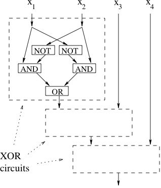
A circuit ${C}$ has ${n}$ inputs, ${m}$ outputs, and is constructed with AND gates, OR gates and NOT gates. Each gate has in-degree 2 except the NOT gate which has in-degree 1. The out-degree can be any number. A circuit must have no cycle. The following picture shows an example of a boolean circuit computing the function ${f(x_1 x_2 x_3 x_4) = x_1 \oplus x_2 \oplus x_3 \oplus x_4}$

Define ${{\bf SIZE}(C) = \#}$ of AND and OR gates of ${C}$ . By convention, we do not count the NOT gates.

To be compatible with other complexity classes, we need to extend the model to arbitrary input sizes:

Definition 1 A language ${L}$ is solved by a family of circuits ${\{C_1, C_2, \ldots, C_n, \ldots\}}$ if for every ${n \geq 1}$ and for every ${x}$ s.t. ${|x| = n}$ ,

$\displaystyle x \in L \,\, \iff \,\, f_{C_n}(x)=1.$

Definition 2 Say ${L \in {\bf SIZE}(s(n))}$ if ${L}$ is solved by a family ${\{C_1, C_2, \ldots, C_n, \ldots\}}$ of circuits, where ${C_i}$ has at most ${s(i)}$ gates.

2. Relation to other complexity classes

Unlike other complexity measures, like time and space, for which there are languages of arbitrarily high complexity, the size complexity of a problem is always at most exponential.

Theorem 3 For every language ${L}$ , ${L \in {\bf SIZE}(O(2^n))}$ .

Proof: We need to show that for every 1-output function ${f:\{ 0,1 \}^n \rightarrow \{ 0,1 \}}$ , ${f}$ has circuit size ${O(2^n)}$ .

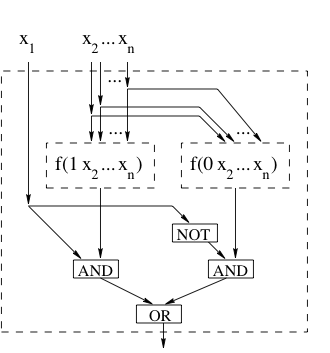
Use the identity ${f(x_1 x_2 \ldots x_n) = (x_1 \land f(1 x_2 \ldots x_n)) \lor (\overline{x}_1 \land f(0 x_2 \ldots x_n))}$ to recursively construct a circuit for ${f}$ , as shown in the figure below

The recurrence relation for the size of the circuit is: ${s(n) = 3 + 2s(n-1)}$ with base case ${s(1) = 1}$ , which solves to ${s(n) = 2 \cdot 2^n - 3 = O(2^n)}$ . $\Box$

The exponential bound is nearly tight.

Theorem 4 There are languages ${L}$ such that ${L \not\in {\bf SIZE}(o(2^{n}/n))}$ . In particular, for every ${n\geq 11}$ , there exists ${f:\{ 0,1 \}^n \rightarrow \{ 0,1 \}}$ that cannot be computed by a circuit of size ${2^n/4n}$ .

Proof: This is a counting argument. There are ${2^{2^n}}$ functions ${f:\{ 0,1 \}^n \rightarrow \{ 0,1 \}}$ , and we claim that the number of circuits of size ${s}$ is at most ${2^{O(s \log s)}}$ , assuming ${s \geq n}$ . To bound the number of circuits of size ${s}$ we create a compact binary encoding of such circuits. Identify gates with numbers ${1,\ldots,s}$ . For each gate, specify where the two inputs are coming from, whether they are complemented, and the type of gate. The total number of bits required to represent the circuit is

$\displaystyle s\times (2 \log (n+s) + 3) \leq s\cdot (2 \log 2s + 3) = s\cdot (2 \log 2s + 5).$

So the number of circuits of size ${s}$ is at most ${2^{2s \log s + 5s}}$ , and this is not sufficient to compute all possible functions if

$\displaystyle 2^{2s \log s + 5s} < 2^{2^n}.$

This is satisfied if ${s \leq \frac {2^n}{4n}}$ and ${n\geq 11}$ . $\Box$

The following result shows that efficient computations can be simulated by small circuits.

Theorem 5 If ${L \in {\bf DTIME}(t(n))}$ , then ${L \in {\bf SIZE}(O(t^2(n)))}$ .

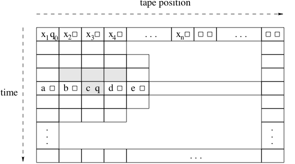
Proof: Let ${L}$ be a decision problem solved by a machine ${M}$ in time ${t(n)}$ . Fix ${n}$ and ${x}$ s.t. ${|x| = n}$ , and consider the ${t(n) \times t(n)}$ tableau of the computation of ${M(x)}$ . See the figure below.

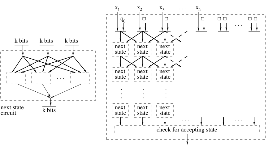
Assume that each entry ${(a,q)}$ of the tableau is encoded using ${k}$ bits. By Proposition 3, the transition function ${\{ 0,1 \}^{3k} \rightarrow \{ 0,1 \}^k}$ used by the machine can be implemented by a “next state circuit” of size ${k \cdot O(2^{3k})}$ , which is exponential in ${k}$ but constant in ${n}$ . This building block can be used to create a circuit of size ${O(t^2(n))}$ that computes the complete tableau, thus also computes the answer to the decision problem. The complete construction is shown in the figure below.

$\Box$

Corollary 6 ${{\bf P} \subseteq {\bf SIZE}(n^{O(1)})}$ .

On the other hand, it’s easy to show that ${{\bf P} \neq {\bf SIZE}(n^{O(1)})}$ , and, in fact, one can define languages in ${{\bf SIZE}(O(1))}$ that are undecidable.

3. Randomized Algorithms

First we are going to describe the probabilistic model of computation. In this model an algorithm ${A}$ gets as input a sequence of random bits ${r}$ and the ”real” input ${x}$ of the problem. The output of the algorithm is the correct answer for the input ${x}$ with some probability.

Definition 7 An algorithm ${A}$ is called a polynomial time probabilistic algorithm if the size of the random sequence ${|r|}$ is polynomial in the input ${|x|}$ and ${A()}$ runs in time polynomial in ${|x|}$ .

If we want to talk about the correctness of the algorithm, then informally we could say that for every input ${x}$ we need ${\mathop{\mathbb P}[ A(x,r)=\text{correct answer for } x] \geq \frac{2}{3}}$ . That is, for every input the probability distribution over all the random sequences must be some constant bounded away from ${\frac{1}{2}}$ . Let us now define the class BPP.

Definition 8 A decision problem ${L}$ is in ${{\bf BPP}}$ if there is a polynomial time algorithm ${A}$ and a polynomial ${p()}$ such that :

$\displaystyle \forall x\in L \;\;\; \mathop{\mathbb P}_{r\in \{0,1\}^{p(|x|)}}[A(x,r)=1] \geq 2/3$

$\displaystyle \forall x\not\in L\;\;\; \mathop{\mathbb P}_{r\in \{0,1\}^{p(|x|)}}[A(x,r)=1] \leq 1/3$

We can see that in this setting we have an algorithm with two inputs and some constraints on the probabilities of the outcome. In the same way we can also define the class P as:

Definition 9 A decision problem ${L}$ is in ${{\bf P}}$ if there is a polynomial time algorithm ${A}$ and a polynomial ${p()}$ such that :

$\displaystyle \forall x\in L \;\;\; : \mathop{\mathbb P}_{r\in \{0,1\}^{p(|x|)}}[A(x,r)=1] =1$

$\displaystyle \forall x\not\in L : \mathop{\mathbb P}_{r\in \{0,1\}^{p(|x|)}}[A(x,r)=1] = 0$

Similarly, we define the classes ${{\bf RP}}$ and ZPP.

Definition 10 A decision problem ${L}$ is in ${{\bf RP}}$ if there is a polynomial time algorithm ${A}$ and a polynomial ${p()}$ such that:

$\displaystyle \forall x\in L \;\;\; \mathop{\mathbb P}_{r\in \{0,1\}^{p(|x|)}}[A(x,r)=1] \geq 1/2$

$\displaystyle \forall x\not\in L \;\;\; \mathop{\mathbb P}_{r\in \{0,1\}^{p(|x|)}}[A(x,r)=1] \leq 0$

Definition 11 A decision problem ${L}$ is in ${{\bf ZPP}}$ if there is a polynomial time algorithm ${A}$ whose output can be ${0,1,?}$ and a polynomial ${p()}$ such that :

$\displaystyle \forall x \;\;\; \mathop{\mathbb P}_{r\in \{0,1\}^{p(|x|)}}[A(x,r)=?] \leq 1/2$

$\displaystyle \forall x, \forall r\;\;\; \text{such that}\;\;\; A(x,r)\neq ? . ( \ A(x,r)=1 \;\;\; \Leftrightarrow \;\;\; x\in L \ )$

4. Relations between complexity classes

After defining these probabilistic complexity classes, let us see how they are related to other complexity classes and with each other.

Theorem 12 RP ${\subseteq}$ NP.

Proof: Suppose we have a ${{\bf RP}}$ algorithm for a language ${L}$ . Then this algorithm is can be seen as a “verifier” showing that ${L}$ is in NP. If ${x \in L}$ then there is a random sequence ${r}$ , for which the algorithm answers yes, and we think of such sequences ${r}$ as witnesses that ${x\in L}$ . If ${x \not\in L}$ then there is no witness. $\Box$

We can also show that the class ZPP is no larger than RP.

Theorem 13 ZPP ${\subseteq}$ RP.

Proof: We are going to convert a ZPP algorithm into an RP algorithm. The construction consists of running the ZPP algorithm and anytime it outputs ${?}$ , the new algorithm will answer ${0}$ . In this way, if the right answer is ${0}$ , then the algorithm will answer ${0}$ with probability ${1}$ . On the other hand, when the right answer is ${1}$ , then the algorithm will give the wrong answer with probability less than ${1/2}$ , since the probability of the ZPP algorithm giving the output ${?}$ is less than ${1/2}$ . $\Box$

Another interesting property of the class ZPP is that it’s equivalent to the class of languages for which there is an average polynomial time algorithm that always gives the right answer. More formally,

Theorem 14 A language ${L}$ is in the class ${{\bf ZPP}}$ if and only if ${L}$ has an average polynomial time algorithm that always gives the right answer.

Proof: First let us clarify what we mean by average time. For each input ${x}$ we take the average time of ${A(x,r)}$ over all random sequences ${r}$ . Then for size ${n}$ we take the worst time over all possible inputs ${x}$ of size ${|x|=n}$ . In order to construct an algorithm that always gives the right answer we run the ${{\bf ZPP}}$ algorithm and if it outputs a ${?}$ , then we run it again. Suppose that the running time of the ${{\bf ZPP}}$ algorithm is ${T}$ , then the average running time of the new algorithm is:

$\displaystyle T_{avg}=\frac{1}{2}\cdot T+\frac{1}{4}\cdot 2T+\ldots+\frac{1}{2^k}\cdot kT = O(T)$

Now, we want to prove that if the language ${L}$ has an algorithm that runs in polynomial average time ${t(|x|)}$ , then this is in ZPP. We run the algorithm for time ${2t(|x|)}$ and output a ${?}$ if the algorithm has not yet stopped. It is straightforward to see that this belongs to ZPP. First of all, the worst running time is polynomial, actually ${2t(|x|)}$ . Moreover, the probability that our algorithm outputs a ${?}$ is less than ${1/2}$ , since the original algorithm has an average running time ${t(|x|)}$ and so it must stop before time ${2t(|x|)}$ at least half of the times. $\Box$

Let us now prove the fact that ${{\bf RP}}$ is contained in BPP.

Theorem 15 RP ${\subseteq}$ BPP

Proof: We will convert an ${{\bf RP}}$ algorithm into a ${{\bf BPP}}$ algorithm. In the case that the input ${x}$ does not belong to the language then the ${{\bf RP}}$ algorithm always gives the right answer, so it certainly satisfies that ${{\bf BPP}}$ requirement of giving the right answer with probability at least ${2/3}$ . In the case that the input ${x}$ does belong to the language then we need to improve the probability of a correct answer from at least ${1/2}$ to at least ${2/3}$ .

Let ${A}$ be an RP algorithm for a decision problem ${L}$ . We fix some number ${k}$ and define the following algorithm:

input: ${x}$ ,
pick ${r_1,r_2,\ldots,r_k}$
if ${A(x,r_1)=A(x,r_2)=\ldots=A(x,r_k)=0}$ then return 0
else return 1

Let us now consider the correctness of the algorithm. In case the correct answer is ${0}$ the output is always right. In the case where the right answer is ${1}$ the output is right except when all ${A(x,r_i)=0}$ .

$\displaystyle \text{if} \;\;\;x\not\in L\;\;\; \mathop{\mathbb P}_{r_1,\ldots,r_k}[A^k(x,r_1,\ldots,r_k)=1] = 0$

$\displaystyle \text{if}\;\;\; x\in L\;\;\; \mathop{\mathbb P}_{r_1,\ldots,r_k}[A^k(x,r_1,\ldots,r_k)=1] \geq 1-\left(\dfrac{1}{2}\right)^k$

It is easy to see that by choosing an appropriate ${k}$ the second probability can go arbitrarily close to ${1}$ . In particular, choosing ${k=2}$ suffices to have a probability larger than ${2/3}$ , which is what is required by the definition of BPP. In fact, by choosing ${k}$ to be a polynomial in ${|x|}$ , we can make the probability exponentially close to ${1}$ . This means that the definition of ${{\bf RP}}$ that we gave above would have been equivalent to a definition in which, instead of the bound of ${1/2}$ for the probability of a correct answer when the input is in the language ${L}$ , we had have a bound of ${1-\left(\tfrac{1}{2}\right)^{q(|x|)}}$ , for a fixed polynomial ${q}$ . $\Box$

Let, now, A be a BPP algorithm for a decision problem ${L}$ . Then, we fix ${k}$ and define the following algorithm:

input: ${x}$
pick ${r_1,r_2,\ldots,r_k}$
${c=\sum_{i=1}^k A(x,r_i)}$
if ${c\geq\tfrac{k}{2}}$ then return 1
else return 0

In a BPP algorithm we expect the right answer to come up with probability more than ${1/2}$ . So, by running the algorithm many times we make sure that this slightly bigger than ${1/2}$ probability will actually show up in the results.

We will prove next time that the error probability of algorithm ${A^{(k)}}$ is at most ${2^{-\Omega(k)}}$ .

Enter your comment here...

Fill in your details below or click an icon to log in:

Email (required) (Address never made public)

Name (required)

Website

You are commenting using your WordPress.com account. ( Log Out / Change )

You are commenting using your Twitter account. ( Log Out / Change )

You are commenting using your Facebook account. ( Log Out / Change )

Cancel

Connecting to %s

in theory

"Marge, I agree with you – in theory. In theory, communism works. In theory." — Homer Simpson

CS254 Lecture 3 – Boolean Circuits

Leave a Reply

Share this:

Like this:

Related

Leave a Reply