Today I would like to discuss the Khot-Naor approximation algorithm for the 3-XOR problem, and an open question related to it.
The Khot-Naor Approximation Algorithm for 3-XOR
1

Today I would like to discuss the Khot-Naor approximation algorithm for the 3-XOR problem, and an open question related to it.
Scribed by Rachel Lawrence
In which we introduce semidefinite programming and apply it to Max Cut.
1. Overview
We begin with an introduction to Semidefinite Programming (SDP). We will then see that, using SDP, we can find a cut with the same kind of near-optimal performance for Max Cut in random graphs as we got from the greedy algorithm — that is,
in random graphs 

with high probability in
Methods using SDP will become particularly helpful in future lectures when we consider planted-solution models instead of fully random graphs: greedy algorithms will fail on some analogous problems where methods using SDP can succeed.
2. Semidefinite Programming
Semidefinite Programming (SDP) is a form of convex optimization, similar to linear programming but with the addition of a constraint stating that, if the variables in the linear program are considered as entries in a matrix, that matrix is positive semidefinite. To formalize this, we begin by recalling some basic facts from linear algebra.
2.1. Linear algebra review
Definition 1 (Positive Semidefinite) A matrix
is positive semidefinite (abbreviated PSD and written
) if it is symmetric and all its eigenvalues are non-negative.
We will also make use of the following facts from linear algebra:
 is a symmetric matrix, then all the eigenvalues of
  are real, and, if we call
  the eigenvalues of with repetition, we have
where the 

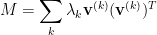
has the characterization
and the optimization problem in the right-hand side is solvable up to arbitrarily good accuracy
This gives us the following lemmas:
Lemma 2
we have
.
Proof: From part (2) above, the smallest eigenvalue of M is given by
Noting that we always have 


Lemma 3 If
, then

Proof: 


Lemma 4 If
and
, then

Proof: 

2.2. Formulation of SDP
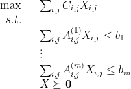
With these characterizations in mind, we define a semidefinite program as an optimization program in which we have 


where the matrices 

We will also use the following alternative characterization of PSD matrices
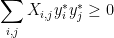
Lemma 5 A matrix
such that, for every
, we have
.
Proof: Suppose that 

Conversely, if
we have
and we see that we can define 

and we do have the property that
This leads to the following equivalent formulation of the SDP optimization problem:
where our variables are vectors
2.3. Polynomial time solvability
From lemmas 3 and 4, we recall that if 


Using the ellipsoid algorithm, one can solve in polynomial time (up to arbitrarily good accuracy) any optimization problem in which one wants to optimize a linear function over a convex feasible region, provided that one has a separation oracle for the feasible region: that is, an algorithm that, given a point,
In order to construct a separation oracle for a SDP, it is enough to solve the following problem: given a matrix 
and that the above minimization problem is solvable in polynomial time (up to arbitrarily good accuracy). If the above optimization problem has a non-negative optimum, then 
is satisfied for all PSD matrices 
3. SDP Relaxation of Max Cut and Random Hyperplane Rounding
The Max Cut problem in a given graph 

We can interpret this as associating every vertex 


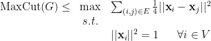
While quadratic optimization is NP-hard, we can instead use a relaxation to a polynomial-time solvable problem. We note that any quadratic optimization problem has a natural relaxation to an SDP, in which we relax real variables to take vector values and we change multiplication to inner product:

Figure 1: The hyperplane through the origin defines a cut partitioning the vertices into sets 

Solving the above SDP, which is doable in polynomial time up to arbitrarily good accuracy, gives us a unit vector 


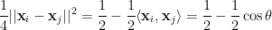
Let 


and the contribution of
Some calculus shows that for every 
and so
so we have a polynomial time approximation algorithm with worst-case approximation guarantee 
Next time, we will see how the SDP relaxation behaves on random graphs, but first let us how it behaves on a large class of graphs.
4. Max Cut in Bounded-Degree Triangle-Free Graphs
Theorem 6 If
is a triangle-free graph in which every vertex has degree at most
, then
Proof: Consider the following feasible solution for the SDP: we associate to each node 


For example, if we have a graph such that vertex 1 is adjacent to vertices 3 and 5:
 |
2 | 3 | 4 | 5 |  |
|
 |
 |
0 | ![{-\frac{1}{\sqrt[]{2deg(1)}}}](https://s0.wp.com/latex.php?latex=%7B-%5Cfrac%7B1%7D%7B%5Csqrt%5B%5D%7B2deg%281%29%7D%7D%7D&bg=ffffff&fg=000000&s=0&c=20201002) |
0 | |
|
 |
0 | |
0 | 0 | 0 | |
 |
![{-\frac{1}{\sqrt[]{2deg(3)}}}](https://s0.wp.com/latex.php?latex=%7B-%5Cfrac%7B1%7D%7B%5Csqrt%5B%5D%7B2deg%283%29%7D%7D%7D&bg=ffffff&fg=000000&s=0&c=20201002) |
0 | |
0 | 0 | |
 |
|
|||||
 |
0 | 0 | 0 | 0 | 0 | |
Let us transform this SDP solution into a cut
We see that, for every edge
The probability that
and
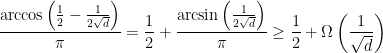
so that the expected number of cut edges is at least 
Cui Peng of Renmin University in Beijing has recently released two preprints, one claiming a proof of P=NP and one claiming a refutation of the Unique Games Conjecture; I will call them the “NP paper” and the “UG paper,” respectively.
Of all the papers I have seen claiming a resolution of the P versus NP problem, and, believe me, I have seen a lot of them, these are by far the most legit. On Scott Aronson’s checklist of signs that a claimed mathematical breakthrough is wrong, they score only two.
Unfortunately, both papers violate known impossibility results.
The two papers follow a similar approach: a certain constraint satisfaction problem is proved to be approximation resistant (under the assumption that P
In both papers, the approximation algorithm is by Hast, and it is based on a semidefinite programming relaxation studied by Charikar and Wirth.
The reason why the results cannot be correct is that, in both cases, if the hardness result is correct, then it implies an integrality gap for the Charikar-Wirth relaxation, which makes it unsuitable to break the approximation resistance as claimed.
Suppose that we have a constraint satisfaction problem in which every constraint is satisfied by a 


For algorithms that are based on relaxations, such certificates came from the relaxation itself: one shows that the algorithm satisfies a number of constraints that is at least 
In the UG paper, the approximation resistance relies on a result of Austrin and Håstad. Like all UGC-based inapproximability results that I am aware of, the hardness results of Austrin and Håstad are based on a long code test. A major result of Raghavendra is that for every constraint satisfaction problem one can write a certain SDP relaxation such that the integrality gap of the relaxation is equal to the ratio between soundness and completeness in the best possible long code test that uses predicates from the constraint satisfaction problem. In particular, in Section 7.7 of his thesis, Prasad shows that if you have a long code test with soundness 


The NP paper adopts a technique introduced by Siu On Chan to prove inapproximability results by starting from a version of the PCP theorem and then applying a “hardness amplification” reduction. Tulsiani proves that if one proves a hardness-of-approximation result via a “local” approximation-reduction from Max 3LIN, then the hardness-of-approximation result is matched by an integrality gap for Lasserre SDP relaxations up to a super-constant number of rounds. The technical sense in which the reduction has to be “local” is as follows. A reduction from Max 3LIN (the same holds for other problems, but we focus on starting from Max 3LIN for concreteness) to another constraint satisfaction problems has two parameters: a “completeness” parameter
to instances of the target problem in which the optimum is at least  ;
;
 to instances of the target problem in which the optimum is at most
  .
.
Since we know that it’s NP-hard to distinguish Max 3LIN instances in which the optimum is
The Bulletin of the AMS has an extensive 87-page survey article on Grothendieck’s inequality in the theory of Banach spaces, and on how it shows up in several contexts, including the use of semidefinite programming to approximate graph partitioning problems.
In which we introduce the Arora-Rao-Vazirani relaxation of sparsest cut, and discuss why it is solvable in polynomial time.
![\displaystyle cut > \frac{|E|}{2} + \Omega(n\cdot\sqrt[]{d})](https://s0.wp.com/latex.php?latex=%5Cdisplaystyle+cut+%3E+%5Cfrac%7B%7CE%7C%7D%7B2%7D+%2B+%5COmega%28n%5Ccdot%5Csqrt%5B%5D%7Bd%7D%29&bg=ffffff&fg=000000&s=0&c=20201002)
![\displaystyle max\ cut < \frac{|E|}{2} + O(n\cdot \sqrt[]{d})](https://s0.wp.com/latex.php?latex=%5Cdisplaystyle+max%5C+cut+%3C+%5Cfrac%7B%7CE%7C%7D%7B2%7D+%2B+O%28n%5Ccdot+%5Csqrt%5B%5D%7Bd%7D%29&bg=ffffff&fg=000000&s=0&c=20201002)


![\displaystyle \mathop{\mathbb P} [ (i,j) \mbox{ is cut } ] = \frac {\theta}{\pi}](https://s0.wp.com/latex.php?latex=%5Cdisplaystyle++%5Cmathop%7B%5Cmathbb+P%7D+%5B+%28i%2Cj%29+%5Cmbox%7B+is+cut+%7D+%5D+%3D+%5Cfrac+%7B%5Ctheta%7D%7B%5Cpi%7D+&bg=ffffff&fg=000000&s=0&c=20201002)
![\displaystyle \mathop{\mathbb E} [ \mbox{ number of edges cut by } (S,V-S) ] \geq .878 \cdot \sum_{(i,j) \in E} \frac 14 || {\bf x}_i - {\bf x}_j ||^2](https://s0.wp.com/latex.php?latex=%5Cdisplaystyle++%5Cmathop%7B%5Cmathbb+E%7D+%5B+%5Cmbox%7B+number+of+edges+cut+by+%7D+%28S%2CV-S%29+%5D+%5Cgeq+.878+%5Ccdot+%5Csum_%7B%28i%2Cj%29+%5Cin+E%7D+%5Cfrac+14+%7C%7C+%7B%5Cbf+x%7D_i+-+%7B%5Cbf+x%7D_j+%7C%7C%5E2+&bg=ffffff&fg=000000&s=0&c=20201002)