In which we introduce the Leighton-Rao relaxation of sparsest cut.
Let  be an undirected graph. Unlike past lectures, we will not need to assume that
  is regular. We are interested in finding a sparsest cut in , where the sparsity of a non-trivial bipartition
  of the vertices is
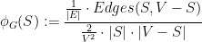
which is the ratio between the fraction of edges that are cut by and the fraction of pairs of vertices that are disconnected by the removal of those edges.
Another way to write the sparsity of a cut is as
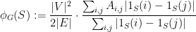
where  is the adjacency matrix of and
  is the indicator function of the set
  .
.
The observation that led us to see  as the optimum of a continuous relaxation of
  was to observe that
  , and then relax the problem by allowing arbitrary functions
  instead of indicator functions
  .
.
The Leighton-Rao relaxation of sparsest cut is obtained using, instead, the following observation: if, for a set , we define  , then
  defines a semi-metric over the set
  , because
  is symmetric,
  , and the triangle inequality holds. So we could think about allowing arbitrary semi-metrics in the expression for , and define
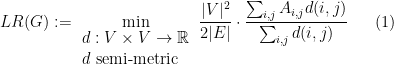
This might seem like such a broad relaxation that there could be graphs on which  bears no connection to
  . Instead, we will prove the fairly good estimate

Furthermore, we will show that , and an optimal solution  can be computed in polynomial time, and the second inequality above has a constructive proof, from which we derive a polynomial time
  -approximate algorithm for sparsest cut.
1. Formulating the Leighton-Rao Relaxation as a Linear Program
The value and an optimal can be computed in polynomial time by solving the following linear program

that has a variable  for every unordered pair of distinct vertices
  . Clearly, every solution to the linear program (3) is also a solution to the right-hand side of the definition (1) of the Leighton-Rao parameter, with the same cost. Also every semi-metric can be normalized so that
 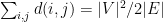 by multiplying every distance by a fixed constant, and the normalization does not change the value of the right-hand side of (1); after the normalization, the semimetric is a feasible solution to the linear program (3), with the same cost.
In the rest of this lecture and the next, we will show how to round a solution to (3) into a cut, achieving the logarithmic approximation promised in (2).
2. An L1 Relaxation of Sparsest Cut
In the Leighton-Rao relaxation, we relax distance functions of the form  to completely arbitrary distance functions. Let us consider an intermediate relaxation, in which we allow distance functions that can be realized by an embedding of the vertices in an
  space.
Recall that, for a vector  , its norm is defined as
  , and that this norm makes
  into a metric space with the distance function

The distance function is an example of a distance function that can be realized by mapping each vertex to a real vector, and then defining the distance between two vertices as the norm of the respective vectors. Of course it is an extremely restrictive special case, in which the dimension of the vectors is one, and in which every vertex is actually mapping to either zero or one. Let us consider the relaxation of sparsest cut to arbitrary mappings, and define

This may seem like another very broad relaxation of sparsest cut, whose optimum might bear no correlation with the sparsest cut optimum. The following theorem shows that this is not the case.
Theorem 1 For every graph ,  .
.
Furthermore, there is a polynomial time algorithm that, given a mapping  , finds a cut such that
Proof: We use ideas that have already come up in the proof the difficult direction of Cheeger’s inequality. First, we note that for every nonnegative reals  and positive reals
  we have

as can be seen by noting that

Let  be the
  -th coordinate of the vector
  , thus
  . Then we can decompose the right-hand side of (4) by coordinates, and write


This already shows that, in the definition of  , we can map, with no loss of generality, to 1-dimensional spaces.
Let  be the coordinate that achieves the minimum above. Because the cost function is invariant under the shifts and scalings (that is, the cost of a function
  is the same as the cost of
  for every two constants
  and
and  ) there is a function
  such that
  has the same cost function as
  and it has a unit-length range
  .
.
Let us now pick a threshold  uniformly at random from the interval
 ![{[\min_v g(v) , \max_v g(v)]}](https://s0.wp.com/latex.php?latex=%7B%5B%5Cmin_v+g%28v%29+%2C+%5Cmax_v+g%28v%29%5D%7D&bg=ffffff&fg=000000&s=0&c=20201002) , and define the random variables
, and define the random variables

We observe that for every pairs of vertices  we have

and so we get
Finally, by an application of (5), we see that there must be a set among the possible values of  such that (4) holds. Notice that the proof was completely constructive: we simply took the coordinate
  of
of  with the lowest cost function, and then the “threshold cut” given by with the smallest sparsity.
3. A Theorem of Bourgain
We will derive our main result (2) from the L1 “rounding” process of the previous section, and from the following theorem of Bourgain (the efficiency considerations are due to Linial, London and Rabinovich).
Theorem 2 (Bourgain) Let  be a semimetric defined over a finite set . Then there exists a mapping
  such that, for every two elements
  ,
,

where  is an absolute constant. Given
  , the mapping can be found with high probability in randomized polynomial time in
  .
.
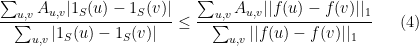
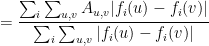
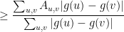
To see that the above theorem of Bourgain implies (2), consider a graph , and let be the optimal solution of the Leighton-Rao relaxation of the sparsest cut problem on , and let  be a mapping as in Bourgain’s theorem applied to . Then


 is the set of natural numbers. The advantage of ILPs is that they are a very expressive language to formulate optimization problems, and they can capture in a natural and direct way a large number of combinatorial optimization problems. The disadvantage of ILPs is that they are a very expressive language to formulate combinatorial optimization problems, and finding optimal solutions for ILPs is NP-hard.
 ;
;  , and so we have found an optimal solution for the ILP and hence an optimal solution for our combinatorial optimization problem;
  has fractional values, but we have a rounding procedure that transforms
  such that
  for some constant
  , and so we have a
 ,
,  ,
,  ,
,  of cost
  . How can we convince ourselves, or another user, that the solution is indeed optimal, without having to trace the steps of the computation of the algorithm?


 we also have
 , add the second inequality, and then add the third inequality scaled by
  that is feasible for

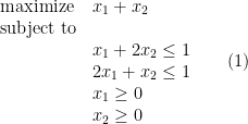
 in the above example) is called the objective function. A feasible solution is an assignment of values to the variables that satisfies the inequalities. The value that the objective function gives to an assignment is called the cost of the assignment. For example,
  and
and  is a feasible solution, of cost
  . Note that if
  are values that satisfy the inequalities, then, by summing the first two inequalities, we see that


