Talagrand’s Generic Chaining

Welcome to phase two of in theory, in which we again talk about math. I spent last Fall teaching two courses and getting settled, I mostly traveled in January and February, and I have spent the last two months on my sofa catching up on TV series. Hence I will reach back to last Spring, when I learned about Talagrand’s machinery of generic chaining and majorizing measures from Nikhil Bansal, in the context of our work with Ola Svensson on graph and hypergraph sparsification. Here I would like to record what I understood about the machinery, and in a follow-up post I plan to explain the application to hypergraph sparsification.

1. A Concrete Setting

Starting from a very concrete setting, suppose that we have a subset ${T \subseteq {\mathbb R}^n}$ , we pick a random Gaussian vector ${g}$ from ${N({\bf 0}, I)}$ , and we are interested in the random variable

$\displaystyle \sup_{t\in T}\ \langle g, t \rangle \ \ \ \ \ (1)$

In theoretical computer science, for example, a random variable like (1) comes up often in the study of rounding algorithms for semidefinite programming, but this is a problem of much broader interest.

We will be interested both in bounds on the expectations of (1) and on its tail, but in this post we will mostly reason about its expectation.

A first observation is that each ${\langle g,t \rangle}$ is Gaussian with mean zero and variance ${|| t||^2}$ . If ${T}$ is finite, we can use a union bound to estimate the tail of ${\sup_{t\in T} \langle t,g \rangle}$ as

$\displaystyle \Pr \left[ \sup_{t\in T}\ \langle g, t \rangle > \ell \right] \leq |T| \cdot e^{-\ell^2 / 2 \sup_{t\in T} ||t||^2}$

and we can compute the upper bound

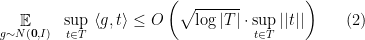
$\displaystyle \mathop{\mathbb E}_{g\sim N({\bf 0}, I)} \ \ \sup_{t\in T}\ \langle g, t \rangle \leq O\left(\sqrt{\log |T|} \cdot \sup_{t\in T} || t|| \right) \ \ \ \ \ (2)$

The above bound can be tight, but it is poor if the points of ${T}$ are densely clustered, and it is useless if ${T}$ is infinite.

It is useful to note that, if we fix, arbitrarily, an element ${t_0 \in T}$ , then we have

$\displaystyle \mathop{\mathbb E}_{g\sim N({\bf 0}, I)} \ \ \sup_{t\in T}\ \langle g, t \rangle = \mathop{\mathbb E}_{g\sim N({\bf 0}, I)} \ \ \sup_{t\in T}\ \langle g, t - t_0 \rangle \ \ \ \ \ (3)$

because ${\mathop{\mathbb E} \langle g, t_0 \rangle = 0}$ . The latter expression is nicer to work with because it makes it more explicit that what we are trying to compute is invariant under shifts of ${T}$ , and only depends on pairwise distances of the elements of ${T}$ , rather than their norm.

In the cases in which (2) gives a poor bound, a natural approach is to reason about an ${\epsilon}$ -net ${T'}$ of ${T}$ , that is, a subset ${T'\subseteq T}$ such that for every ${t\in T}$ there is an element ${\pi(t) \in T'}$ such that ${||t - \pi(t) ||\leq \epsilon}$ . Then we can say that

$\displaystyle \mathop{\mathbb E} \sup_t \langle t - t_0, g \rangle = \mathop{\mathbb E} \sup_{t\in T} \langle t - \pi(t) , g \rangle + \langle \pi(t) -t_0, g \rangle$

$\displaystyle \leq \left( \mathop{\mathbb E} \sup_{t\in T} \langle t - \pi(t) , g \rangle \right) + \left( \mathop{\mathbb E} \sup_{t\in T}\langle \pi(t) -t_0, g \rangle \right)$

$\displaystyle \leq O( \sqrt{\log |T|} ) \cdot \sup_{t\in T} ||t-\pi(t) || + \left( \mathop{\mathbb E} \sup_{t'\in T'}\langle t' -t_0, g \rangle \right)$

$\displaystyle \leq O\left( \sqrt{\log |T|} \cdot \epsilon + \sqrt {\log |T'|} \cdot \sup_{t'\in T'} || t' - t_0|| \right)$

which can be a much tighter bound. Notice that we used (2) to bound

$\displaystyle \mathop{\mathbb E} \sup_{t\in T'} \langle t' - t_0 , g\rangle \ ,$

but it might actually be better to find an ${\epsilon'}$ -net ${T''}$ of ${T'}$ , and so on. In general, a tighter analysis would be to choose a sequence of nested sets ${T_0 \subseteq T_1 \subseteq \cdots \subseteq T_k}$ , where ${T_0 = \{ t_0 \}}$ , ${T_k = T}$ , and we have that ${T_{i-1}}$ is an ${\epsilon_i}$ -net of ${T_{i}}$ , that is, for every element ${t_{i}}$ of ${T_i}$ there is an element ${\pi_i (t_i) \in T_{i-1}}$ such that ${|| t_i - \pi_i (t_i) || \leq \epsilon_i}$ . Then, by generalizing the above reasoning, we get

$\displaystyle \mathop{\mathbb E} \sup_{t\in T} \langle t-t_0,g \rangle \leq O(1) \cdot \sum_{i=1}^k \sqrt{\log |T_i | } \cdot \sup_{t_i \in T_i} || t_i - \pi_i(t_i) || \leq O(1) \cdot \sum_{i=1}^n \epsilon_i \sqrt{\log |T_i | }$

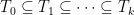
Finally, if the cardinality of the ${T_i}$ grows sufficiently fast, namely, if we have ${|T_i| > |T_{i-1}|^2}$ , it is possible to refine the estimate to

$\displaystyle \mathop{\mathbb E} \sup_{t\in T} \langle t-t_0,g \rangle \leq O(1) \cdot \sup_{t\in T} \sum_{i=1}^k \sqrt{\log |T_i | } \cdot || t - \pi_i (t) ||$

where ${\pi_i(t)}$ is the closest element to ${t}$ in ${T_{i-1}}$ . This is done by avoiding to write the expectation of the sup of a sum as a sum of expectations of sups and then using (2), but by bounding the tail of the sup of the sum directly.

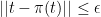
At this point, we do not even need to assume that ${T_k= T}$ , that ${T}$ is finite, or that the sequence of sets is finite, and we have the following result.

Theorem 1 (Talagrand’s generic chaining inequality) Let ${T \subseteq {\mathbb R}^n}$ be an arbitrary set, let ${T_0 \subseteq T_1 \subseteq \cdots T_k \subseteq \cdots \subseteq T}$ be a countable sequence of finite subsets of ${T}$ such that ${|T_0| = 1}$ and ${|T_k| \leq 2^{2^k}}$ . Then

$\displaystyle \mathop{\mathbb E} \sup_{t\in T} \langle t, g \rangle \leq O(1) \cdot \sup_{t\in T} \sum_{k=1}^\infty 2^{k/2} || t - \pi_k(t)||$

where ${\pi_k(t)}$ is the element of ${T_{k-1}}$ closest to ${t}$ .

A short complete proof is in these notes by James Lee.

While the above Theorem has a very simple proof, the amazing thing, which is rather harder to prove, is that it is tight, in the sense that for every ${T}$ there is a sequence of sets such that the bound of the above theorem has a matching lower bound, up to an absolute constant. This is why it is called generic chaining. Chaining because the projection ${\langle t-t_0,g\rangle}$ of ${t-t_0}$ on ${g}$ is estimated based on the “chain”

$\displaystyle \sum_k \langle \pi_{k+1} (t) - \pi_k(t) , g \rangle$

of projections of the intermediate steps of a path that goes from ${t}$ to ${t_0}$ passing through the ${\pi_k(t)}$ . Generic because this upper bound technique works as well as any other possible upper bound, up to an absolute constant.

2. An Abstract Setting

Let now ${T}$ be a completely arbitrary set, and suppose that we have a distribution ${\cal D}$ over functions ${f: T \rightarrow {\mathbb R}}$ and we want to upper bound

$\displaystyle \mathop{\mathbb E}_{F \sim {\cal D}} \ \ \sup_{t\in T} \ F(t)$

That is, we have a random optimization problem with a fixed feasible set ${T}$ , and we want to know the typical value of the optimum. For example, ${T}$ could be the set of cuts of a vertex set ${V}$ , and ${\cal D}$ describe a distribution of random graphs ${G}$ such that ${F(t)}$ is the number of edges cut in a random graph by the cut ${t}$ . Then the above problem is to estimate the average value of the max cut in the random graphs of the distribution. Or ${T}$ could be the unit sphere ${\{ x \in {\mathbb R}^N : ||x|| = 1 \}}$ and ${\cal D}$ describe a distribution of random Hermitian matrices such that ${F(t)}$ is the quadratic form of a random matrix evaluated at ${t}$ . In this case, the above problem is to estimate the average value of the largest eigenvalue of such a random matrix.

We will call the collection of random variables ${\{ F(t) \}_{t\in T}}$ a random process, where ${F}$ is a random variable distributed according to ${\cal D}$ .

If every ${F(t)}$ , and every finite linear combination ${\sum_{i=1}^k \alpha_i F(t_i)}$ , has a Gaussian distribution, then we say that ${\{ F(t) \}_{t\in T}}$ is a Gaussian process, and if, in addition, ${\mathop{\mathbb E} F(t) = 0}$ for every ${t\in T}$ then we say that it is a centered Gaussian process.

If ${T\subseteq {\mathbb R}^n}$ , and we define ${F(t) = \langle t,g\rangle}$ for a random standard Gaussian ${g\sim N({\bf 0},I)}$ , then ${\{ F(t) \}_{t\in T}}$ is a centered Gaussian process and, in this case, upper bounding ${\mathop{\mathbb E} \sup F(t)}$ is precisely the problem we studied before.

If ${T\subseteq {\mathbb R}^n}$ and ${F(t) = \langle t,g \rangle}$ for a random standard Gaussian ${g}$ , then, for every ${t_1,t_2 \in T}$ , we have

$\displaystyle \mathop{\mathbb E} \left(F(t_1) - F(t_2)\right)^2 = \mathop{\mathbb E}_{g \sim N({\bf 0},I)} \ \ \langle t_1-t_2,g \rangle^2 = ||t_1 - t_2 ||^2$

and, by analogy, if ${\{ F(t) \}_{t\in T}}$ is a centered Gaussian process, we will define the following distance function on ${T}$ :

$\displaystyle d(t_1,t_2 ) := \sqrt{ \mathop{\mathbb E} (F(t_1) - F(t_2))^2}$

If ${\{ F(t) \}_{t\in T}}$ is a centered Gaussian process then one can prove that the above distance function is a semi-metric on ${T}$ .

We will not need this fact, but if ${\{ F(t) \}_{t\in T}}$ is a centered Gaussian process and ${T}$ is finite, then there is an embedding ${h: T \rightarrow {\mathbb R}^n}$ , for some ${n}$ , such that the process can be equivalently defined as picking ${g\sim N({\bf 0} , I)}$ and setting ${F(t) := \langle h(t), g \rangle}$ , so that ${h}$ is also an isometric embedding of the above distance function into ${\ell_2}$ .

The arguments of the previous section apply to centered Gaussian processes without change, and so we have.

Theorem 2 Let ${T}$ be an arbitrary set, and ${\{ F(t) \}_{t\in T}}$ be a centered Gaussian process. Let ${T_0 \subseteq T_1 \subseteq \cdots T_k \subseteq \cdots \subseteq T}$ be a countable sequence of finite subsets of ${T}$ such that ${|T_0| = 1}$ and ${|T_k| \leq 2^{2^k}}$ . Then

$\displaystyle \mathop{\mathbb E} \sup_{t\in T} F(t) \leq O(1) \cdot \sup_{t\in T} \sum_{k=1}^\infty 2^{k/2} d (t , \pi_k(t))$

where ${d(\cdot,\cdot)}$ is the distance function ${d(t_1 , t_2) = \sqrt{ \mathop{\mathbb E} (F(t_1) - F(t_2))^2 }}$ and ${\pi_k(t)}$ is the element of ${T_{k-1}}$ closest to ${t}$ according to ${d(\cdot,\cdot)}$ .

3. Sub-Gaussian Random Processes

This theory does not seem to apply to problems such as bounding the max cut of a ${G_{n,p}}$ unweighted graph, or bounding the largest eigenvalue of a random symmetric matrix with ${\pm 1}$ entries, because such problems have a finite sample space and so cannot be modeled as Gaussian processes.

Fortunately, there is a notion of a sub-Gaussian process, which applies to such problems and which reduces their analysis to the analysis of a related Gaussian process.

First, recall that a centered real-valued random variable ${X}$ is sub-Gaussian if there is a centered Gaussian random variable whose tail dominates the tail of ${X}$ , that is, if we have two constants ${k}$ and ${v}$ such that, for all ${t}$ :

$\displaystyle \Pr [ X \geq t ] \leq k \cdot e^{-t^2 /v }$

An equivalent condition is that there is a ${v}$ such that

$\displaystyle \mathop{\mathbb E} e^{X^2 / v} = O(1)$

In that case, we can define a norm, called the ${\Psi_2}$ norm as

$\displaystyle || X ||_{\Psi_2} := \inf \{ \sigma : \mathop{\mathbb E} e^{X^2 / \sigma^2} \leq 2 \}$

which is, roughly, the standard deviation of a centered Gaussian that dominates ${X}$ .

Example 1 All bounded random variables are sub-Gaussian.

Example 2 If

$\displaystyle X = \sum_i X_i$

where the ${X_i}$ are independent Rademacher random variables, that is, if each ${X_i}$ is equally likely to be +1 or -1, then ${X}$ is sub-Gaussian with ${|| X||_{\Psi_2} = O(\sqrt n)}$ , which is within a constant factor of its actual standard deviation.

Example 3 If

$\displaystyle X = \sum_i X_i$

where the ${X_i}$ are independent and each ${X_i}$ has probability ${p}$ of being equal to ${1-p}$ and probability ${1-p}$ of being equal to ${-p}$ (that is, each ${X_i}$ is a centered Bernoulli random variable), then ${|| X||_{\Psi_2} = \Omega \left( \sqrt {\frac {n} {\log 1/p } } \right)}$ , which is much more than the standard deviation of ${X}$ when ${p}$ is small.

Example 4 If

$\displaystyle X = \sum_i a_i X_i$

where the ${X_i}$ are independent Rademacher random variables, and the ${a_i}$ are arbitrary real scalars, then ${|| X ||_{\Psi_2} = O(\sqrt {\sum_i a_i^2 })}$ , which is within a constant factor of the standard deviation that we would get by replacing each ${X_i}$ with a standard Gaussian.

Let now ${\{ F(t) \}_{t\in T}}$ be a centered random process. We will say that a Gaussian process ${\{ \hat F(t) \}_{t\in T} }$ ${K}$ -dominates ${F}$ if, for every ${t_1,t_2 \in T}$ we have

$\displaystyle || F(t_1) - F(t_2) ||_{\Psi_2} \leq K \cdot \sqrt{\mathop{\mathbb E} \left (\hat F(t_1) - \hat F(t_2) \right)^2 }$

That is, every random variable of the form ${F(t_1) - F(t_2)}$ is sub-Gaussian, and its tail is dominated by the tail of the Gaussian distribution ${\hat F(t_1) - \hat F(t_2)}$

Theorem 3 (Talagrand’s comparison inequality) There is an absolute constant ${C}$ such that if ${\{ F(t) \}_{t\in T}}$ is a centered random process that is ${K}$ -dominated by a centered Gaussian random process ${\{ \hat F(t) \}_{t\in T} }$ , then

$\displaystyle \mathop{\mathbb E} \sup_{t\in T} \ F(t) \leq CK \mathop{\mathbb E} \sup_{t\in T} \hat F(t)$

Furthermore, for every ${\ell \geq 0}$ ,

$\displaystyle \Pr \left[ \sup_{t_1,t_2 \in T} F(t_1) - F(t_2) \geq CK \ \left( \ell \cdot diam(T) + \mathop{\mathbb E} \sup_{t\in T} \hat F(t) \right) \right] \leq 2 e^{-\ell^2} \ ,$

where ${diam(T)}$ is the diameter of ${T}$ with respect to the distance function ${d(s,t) := \sqrt{\mathop{\mathbb E} \left (\hat F(s) - \hat F(t) \right)^2}}$ .

The way to apply this theory is the following.

Suppose that we want estimate, on average or with high probability, the optimum of an optimization problem with feasible set ${T}$ over the randomness of the choice of a random instance. We model this problem like a centered random process ${\{ F(t) \}_{t\in T}}$ in which ${F(t)}$ is the difference between the cost of solution ${t}$ in a random instance minus the average cost of ${t}$ .

Then we think about a related random experiment, in which the random choices involved in constructing our instance are replaced by Gaussian choices (for example, instead of a ${G_{n,1/2}}$ random graph we may think of a complete graph with Gaussian weights on the edges chosen with expectation 1/2 and constant variance) and we let ${\{ \hat F(t) \}_{t\in T}}$ be the analogous process in this Gaussian model.

If we can argue that ${\hat F}$ dominates ${F}$ , then it remains to estimate ${\mathop{\mathbb E} \sup \hat F}$ , which we can do either by the generic chaining theorem or by other methods.

4. An Example

We will now use this machinery to show that the largest eigenvalue of a random symmetric ${n\times n}$ matrix with Rademacher entries is ${O(\sqrt n)}$ . This is certainly not the simplest way of proving such a result, but it will give a sense of how these techniques can be applied.

We let ${T = \{ x\in {\mathbb R}^n : ||x ||=1 \}}$ be the unit sphere.

Our Gaussian process will be to pick standard Gaussians ${g_{i,j}}$ , for each ${1 \leq i \leq j \leq n}$ , define the matrix ${ \hat M_{i,j} = \hat M_{j,i} = g_{i,j}}$ and let

$\displaystyle \hat F(x) = x^T \hat M x$

for every ${x\in T}$ .

Our “sub-Gaussian” random process is to pick Rademacher random variables ${r_{i,j}}$ , for each ${1 \leq i \leq j \leq n}$ , define the matrix ${ M_{i,j} = M_{j,i} = r_{i,j}}$ and let

$\displaystyle F(x) = x^T M x$

for every ${x\in T}$ .

We will argue that ${F}$ is ${O(1)}$ -dominated by ${\hat F}$ and that ${\mathop{\mathbb E} \sup \hat F = O(\sqrt n)}$ .

For the first claim, we see that for every ${x,y \in T}$ , we can write ${F(x)-F(y)}$ as

$\displaystyle F(x) - F(y) = \sum_{i,j} M_{i,j} (x_ix_j - y_iy_j) = 2 \sum_{i<j} r_{i,j} (x_ix_j - y_iy_j) + \sum_i r_{i,i} (x_i^2 - y_i^2)$

So, as noted in one of our examples above, we can say that

$\displaystyle || F(x) - F(y) ||^2_{\Psi_2} \leq O \left( 4 \sum_{i<j} (x_ix_j - y_iy_j) ^2 + \sum_i (x_i^2 - y_i^2)^2 \right)$

and we see that

$\displaystyle (d(x,y))^2 = \mathop{\mathbb E} ( \hat F(x) - \hat F(y) )^2 = 4 \sum_{i<j} (x_ix_j - y_iy_j) ^2 + \sum_i (x_i^2 - y_i^2)^2$

so that, indeed, ${F}$ is ${O(1)}$ -dominated by ${\hat F}$ .

Now we need to apply generic chaining to ${F}$ . It is very helpful to note that the distance function defined on ${T}$ by the Gaussian process is dominated by Euclidean distance between the vectors ${x}$ and ${y}$ , because

$\displaystyle (d(x,y))^2 \leq 2 || xx^T - yy^T ||^2_F \leq 2 \cdot (||x|| + ||y||)^2 \cdot ||x-y||^2 = 8 ||x-y||^2$

where we used the inequality

$\displaystyle || xx^T - yy^T ||_F \leq ( ||x || + ||y||) \cdot ||x-y||$

We can conclude that an ${\epsilon}$ -net over the unit Euclidean sphere is also a ${\sqrt {8}\cdot \epsilon}$ -net for the metric space ${(T,d)}$ . For the unit Euclidean sphere there is an ${\epsilon}$ -net of size at most ${(3/\epsilon)^n}$ . To apply generic chaining, let ${T_k}$ be an arbitrary subset of ${T}$ of cardinality ${2^{2^k}}$ if ${2^k < n}$ , and an ${\epsilon}$ -net with ${\epsilon = 3\cdot 2^{-2^k / n}}$ otherwise. Applying the generic chaining inequality,

$\displaystyle \mathop{\mathbb E} \sup \ \hat F \leq O(1) \cdot \sum_k 2^{k/2} \cdot \sqrt{8} \cdot \min \left\{ 2, 3\cdot 2^{-2^k / n} \right\} = O(\sqrt n)$

8 thoughts on “Talagrand’s Generic Chaining”

Dubayashi on May 3, 2020 at 11:18 am said:

Very nice!
MarioDiaz on May 7, 2020 at 5:44 am said:

Nice post! I think there is a missing parenthesis in the displayed equation defining d(t1,t2).
MarioDiaz on May 7, 2020 at 5:58 am said:

The equation for the definition of the Psi2 norm does not show correctly.
luca on May 7, 2020 at 6:34 am said:

Thanks for the corrections
Pingback: To cheer you up in difficult times 3: A guest post by Noam Lifshitz on the new hypercontractivity inequality of Peter Keevash, Noam Lifshitz, Eoin Long and Dor Minzer | Combinatorics and more
Pingback: Spielman-Srivastava Sparsification à la Talagrand | in theory
Tan on April 9, 2022 at 7:53 am said:

I was wondering, how do you obtain the bound for (2) when T is finite? I guess you integrate P(X > l) but I was wondering if there was a trick to get that bound?
Pingback: An upper bound on Gaussian mean width – Mathematics – Forum

in theory

"Marge, I agree with you – in theory. In theory, communism works. In theory." — Homer Simpson

Talagrand’s Generic Chaining

8 thoughts on “Talagrand’s Generic Chaining”

Leave a comment

Share this:

Related

8 thoughts on “Talagrand’s Generic Chaining”

Leave a comment