CS245 Lecture 6 – Karp-Lipton

In this lecture we prove the Karp-Lipton theorem that if all NP problems have polynomial size circuits then the polynomial hierarchy collapses. A nice application is a theorem of Kannan, showing that, for every {k}, there are languages in {\Sigma_2} requiring circuits of size {\Omega(n^k)}. The next result we wish to prove is that all approximate combinatorial counting problem can be solved within the polynomial hierarchy. Before introducing counting problems and the hashing techniques that will yield this result, we prove the Valiant-Vazirani theorem that solving SAT on instances with exactly one satisfying assignment is as hard as solving SAT in general.

1. The Karp-Lipton Theorem

Theorem 1 (Karp-Lipton) If {{\bf NP} \subseteq {\bf SIZE}(n^{O(1)})} then {\Sigma_2 = \Pi_2} and therefore the polynomial hierarchy would collapse to its second level.

Before proving the above theorem, we first show a result that contains some of the ideas in the proof of the Karp-Lipton theorem.

Lemma 2 If {{\bf NP} \subseteq {\bf SIZE}(n^{O(1)})} then for every polynomial time computable {F(\cdot,\cdot)} and every polynomial {p(\cdot)}, there is a family of polynomial size circuits such that

\displaystyle  C_{|x|}(x) = \left \{ \begin{aligned} y : F(x, y)=1 \qquad \text{ if such a y exists}\\ \text{a sequence of zeroes} \qquad \text{ if otherwise}\\ \end{aligned} \right.

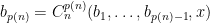
Proof: We define the circuits {C_n^1,\ldots,C_n^{p(n)}} as follows:

{C^i_n}, on input x and bits {b_1,\ldots,b_{i-1}}, outputs 1 if and only if there is a satisfying assignment for {F(x,y) = 1} where {y_1=b_1,\ldots,y_{i-1} = b_{i-1}, y_i=1}.

Also, each circuit realizes an NP computation, and so it can be built of polynomial size. Consider now the sequence {b_1=C^1_n(x)}, {b_2 = C^2_n(b_1,x)}, {\ldots}, {b_{p(n)}=C^{p(n)}_n(b_1,\ldots,b_{p(n)-1},x)}, as shown in the following picture:

The reader should be able to convince himself that this is a satisfying assignment for {F(x,y)=1} if it is satisfiable, and a sequence of zeroes otherwise. \Box

We now prove the Karp-Lipton theorem.

Proof: } We will show that if {{\bf NP} \subseteq {\bf SIZE}(n^{O(1)})} then {\Pi_2 \subseteq \Sigma_2}. By a result in a previous lecture, this implies that {\forall k \geq 2 \;\; \Sigma_k = \Sigma_2}.

Let {L\in \Pi_2}, then there is a polynomial {p(\cdot)} and a polynomial-time computable {F(\cdot)} such that

\displaystyle  x\in L \leftrightarrow \forall y_1.|y_1|\leq p(|x|) \exists y_2 . |y_2| \leq p(|x|). F(x,y_1,y_2)=1

By using Lemma 2, we can show that, for every {n}, there is a circuit {C_n} of size polynomial in {n} such that for every {x} of length {n} and every {y_1}, {|y_1| \leq p(|x|)},

\displaystyle  \exists y_2 . |y_2| \leq p(|x|) \wedge F(x,y_1,y_2) =1 \mbox { if and only if } F(x,y_1,C_n(x,y_1))=1

Let {q(n)} be a polynomial upper bound to the size of {C_n}.

So now we have that for inputs {x} of length {n},

\displaystyle  x\in L \leftrightarrow \exists C .|C| \leq q(n). \forall y_1. |y_1| \leq p(n). F(x,y_1,C(x,y_1))=1

which shows that {L} is in {\Sigma_2}. \Box

2. Kannan’s Theorem

Although it is open to prove that the polynomial hierarchy is not contained in {{\bf P}/poly}, it is not hard to prove the following result.

Theorem 3 For every polynomial {p()}, there is a language {L \in \Sigma_3} such that {L \not\in {\bf SIZE}(p(n))}.

Note that Theorem is not saying that {\Sigma_3 \not\subseteq {\bf P}/poly}, because for that to be true we would have to be able to construct a single language {L} such that for every polynomial {p} we have {L\not\in{\bf SIZE}(p(n))}, instead of constructing a different language for each polynomial. (This is an important difference: the time hierarchy theorem gives us, for every polynomial {p()}, a language {L\in {\bf P}} such that {L\not\in {\bf DTIME}(p(n))}, but this doesn’t mean that {{\bf P} \neq {\bf P}}.)

Kannan observed the following consequence of Theorem 2 and of the Karp-Lipton theorem.

Theorem 4 For every polynomial {p()}, there is a language {L \in \Sigma_2} such that {L \not\in {\bf SIZE}(p(n))}.

Proof: We consider two cases:

  • if {3SAT \not\in {\bf SIZE}(p(n))}; then we are done because {3SAT \in {\bf NP} \subseteq \Sigma_2}.

  • if {3SAT \in {\bf SIZE}(p(n))}, then {{\bf NP}\subseteq {\bf P}/poly}, so by the Karp-Lipton theorem we have {\Sigma_3 = \Sigma_2}, and the language {L \in \Sigma_3 - {\bf SIZE}(p(n))} given by Theorem 2 is in {\Sigma_2}.

\Box

3. The Valiant-Vazirani Theorem

In this section we show the following: suppose there is an algorithm for the satisfiability problem that always find a satisfying assignment for formulae that have exactly one satisfiable assignment (and behaves arbitrarily on other instances): then we can get an RP algorithm for the general satisfiability problem, and so {{\bf NP}={\bf RP}}.

We prove the result by presenting a randomized reduction that given in input a CNF formula {\phi} produces in output a polynomial number of formulae {\psi_0,\ldots,\psi_n}. If {\phi} is satisfiable, then (with high probability) at least one of the {\psi_i} is satisfiable and has exactly one satisfying assignment; if {\phi} is not satisfiable, then (with probability one) all {\psi_i} are unsatisfiable.

The idea for the reduction is the following. Suppose {\phi} is a satisfiable formula with {n} variables that has about {2^k} satisfying assignments, and let {h:\{ 0,1 \}^n \rightarrow \{ 0,1 \}^k} be a hash function picked from a family of pairwise independent hash functions: then the average number of assignments {x} such that {\phi(x)} is true and {h(x)= (0,\ldots,0)} is about one. Indeed, we can prove formally that with constant probability there is exactly one such assignment,\footnote{ For technical reasons, it will be easier to prove that this is the case when picking a hash function {h:\{ 0,1 \}^n \rightarrow \{ 0,1 \}^{k+2}}.} and that there is CNF formula {\psi} (easily constructed from {\phi} and {h}) that is satisfied precisely by that assignment. By doing the above construction for values of {k} ranging from {0} to {n}, we obtain the desired reduction. Details follow.

Definition 5 Let {H} be a family of functions of the form {h:\{ 0,1 \}^n \rightarrow \{ 0,1 \}^m}. We say that {H} is a family of pair-wise independent hash functions if for every two different inputs {x,y\in \{ 0,1 \}^n} and for every two possible outputs {a,b \in \{ 0,1 \}^m} we have

\displaystyle  \mathop{\mathbb P}_{h\in H} [h(x)=a \wedge h(y)=b] = \frac 1 {2^{2m}}

Another way to look at the definition is that for every {x\neq y}, when we pick {h} at random then the random variables {h(x)} and {h(y)} are independent and uniformly distributed. In particular, for every {x\neq y} and for every {a,b} we have {\mathop{\mathbb P}_h[h(x)=a | h(y)=b] = \mathop{\mathbb P}_h[h(x)=a]}.

For {m} vectors {a_1,\ldots,a_m\in \{ 0,1 \}^{m}} and {m} bits {b_1,\ldots,b_m}, define {h_{a_1,\ldots,a_m,b_1,\ldots,b_m}: \{ 0,1 \}^n \rightarrow \{ 0,1 \}^m} as {h_{{\bf a},b}(x) = (a_1\cdot x + b_1,\ldots,a_m \cdot x+b_m)} where {a \cdot x := \Sigma_ia_ix_i \text{ mod } 2}, and let {H_{AFF}} be the family of functions defined this way. Then it is not hard to see that {H_{AFF}} is a family of pairwise independent hash functions.

7 thoughts on “CS245 Lecture 6 – Karp-Lipton

  1. I have made all the corrections that people have suggested in past comments (thanks to all!) and synchronized the pdf files with the versions posted here

  2. No proof of Theorem 3? =(

    Also, a small typo: all occurrences of “Theorem 2” should be “Theorem 3”

  3. Regarding Theorem 3, Kannan first argues directly about \Sigma_4 (not \Sigma_3). Or is there a similarly easy argument that applies to \Sigma_3?

  4. I don’t know what’s the original proof of Kannan, but consider the language where, on input x of length n, I output h(x), where h() is the lexicographically first function among those that (i) depend only on the first 2klog n bits of the input and (ii) have circuit complexity > n^k.

    Then the language is in \Sigma_3, because it is formulated as

    x \in L

    if and only if

    there exists an h (specified as a truth-table of a function on 2klog n bits) such that:

    1) for all circuits C of size less than n^k (operating on 2klog n input bits), C and h compute different functions;

    2) for all functions g smaller than h in lexicographic order, there exists a circuit C of size less than n^k (operating on 2klog n input bits) such that g and C compute the same function

    note that you can check in deterministic polynomial time whether C and g compute the same function.

    What was Kannan’s proof?

  5. What was Kannan’s proof?

    The same, except that he looked at functions on n-bit inputs and so (essentially) used another alternation to check whether C and g compute the same function.

Leave a comment