
Counting Problems
Today we describe counting problems and the class 

1. Counting Classes
[Note: we did not cover most of the material of this section in class.]
Recall that 


Definition 1 If
is the problem that, given
, asks how many
satisfy
.
Observe that an NP-relation 

Unlike for decision problems there is no canonical way to define reductions for counting classes. There are two common definitions.
Definition 2 We say there is a parsimonious reduction from
to
(written
) if there is a polynomial time transformation
such that for all
.
Often this definition is a little too restrictive and we use the following definition instead.
Definition 3
if there is a polynomial time algorithm for

Theorem 4
Proof: Let 


Theorem 5
is
Proof: We show that there is a parsimonious reduction from 


Notice that if a counting problem 

2. Complexity of counting problems
We will prove the following theorem:
Theorem 6 For every counting problem
in
such that
in time polynomial in
and in
, using an oracle for

The theorem says that 
Another remark concerns the following result.
Theorem 7 (Toda) For every
,
.
This implies that 


We first make some observations so that we can reduce the proof to the task of proving a simpler statement.
- It is enough to prove the theorem for
If we have an approximation algorithm for
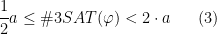
- It is enough to give a polynomial time
-approximation for
Suppose we have an algorithm
such that
Given
, we can construct
where each
is a copy of
satisfying assignments,
has
satisfying assignments. Then, giving
If
,
.
- For a formula
can be found in
.
This can be done by iteratively asking the oracle the questions of the form: “Are there


3. An approximate comparison procedure
Suppose that we had available an approximate comparison procedure a-comp with the following properties:
- If
then
with high probability;
- If
then
with high probability.
Given a-comp, we can construct an algorithm that 
- Input:
- compute:
-
- if
outputs NO from the first time then
- // The value is either
or
and the answer can be checked by one more query to the
- Query to the oracle and output an exact value.
- // The value is either
- else
- Suppose that it outputs YES for
and NO for
- Output
- Suppose that it outputs YES for


We need to show that this algorithm approximates 


and the algorithm outputs the correct answer with in a factor of
Thus, to establish the theorem, it is enough to give a
4. Constructing a-comp
The procedure and its analysis is similar to the Valiant-Vazirani reduction: for a given formula 

In the Valiant-Vazirani reduction, we proved that if 


Lemma 8 Let
be a family of pairwise independent hash functions
. Let
,
. Then,
![\displaystyle \mathop{\mathbb P}_{h\in H} \left[\left| | \{ a\in S: h(a)=0 \} | -\frac{\|S|}{2^m}\right| \geq \epsilon\frac{|S|}{2^m}\right] \leq \frac{1}{4}. \ \ \ \ \ (4)](https://s0.wp.com/latex.php?latex=%5Cdisplaystyle++%5Cmathop%7B%5Cmathbb+P%7D_%7Bh%5Cin+H%7D+%5Cleft%5B%5Cleft%7C+%7C+%5C%7B+a%5Cin+S%3A+h%28a%29%3D0+%5C%7D+%7C+-%5Cfrac%7B%5C%7CS%7C%7D%7B2%5Em%7D%5Cright%7C+%5Cgeq+%5Cepsilon%5Cfrac%7B%7CS%7C%7D%7B2%5Em%7D%5Cright%5D+%5Cleq+%5Cfrac%7B1%7D%7B4%7D.+%5C+%5C+%5C+%5C+%5C+%284%29&bg=ffffff&fg=000000&s=0&c=20201002)
From this, a-comp can be constructed as follows.
- input:
- if
then check exactly whether
.
- if
- pick
, where
- answer YES iff there are more then
assignments
to
.
- pick


Notice that the test at the last step can be done with one access to an oracle to 
- If
, by Lemma 8 we have:
(set
, and
, because
)
which is the success probability of the algorithm.
- If
:
Let
be a superset of
. We have
(by Lemma 8 with
.)
![\displaystyle \mathop{\mathbb P}_{h\in H} \left[\left| \frac{ |S| }{2^m} - | \{a\in S: h(a)=0 \} | \right| \leq \frac{1}{4}\cdot \frac{ |S| }{2^m}\right] \geq \frac{3}{4}](https://s0.wp.com/latex.php?latex=%5Cdisplaystyle++%5Cmathop%7B%5Cmathbb+P%7D_%7Bh%5Cin+H%7D+%5Cleft%5B%5Cleft%7C+%5Cfrac%7B+%7CS%7C+%7D%7B2%5Em%7D+-+%7C+%5C%7Ba%5Cin+S%3A+h%28a%29%3D0+%5C%7D+%7C+%5Cright%7C+%5Cleq+%5Cfrac%7B1%7D%7B4%7D%5Ccdot+%5Cfrac%7B+%7CS%7C+%7D%7B2%5Em%7D%5Cright%5D+%5Cgeq+%5Cfrac%7B3%7D%7B4%7D+&bg=ffffff&fg=000000&s=0&c=20201002)
![\displaystyle \begin{aligned} \mathop{\mathbb P}_{h\in H} \left[ | \{ a\in S: h(a)=0 \} | \geq \frac 34 \cdot \frac{ |S| }{2^m}\right] & \geq \frac{3}{4},\\ \mathop{\mathbb P}_{h\in H} \left[ | \{a\in S: h(a)=0 \} | \geq 48 \right] & \geq \frac{3}{4},\\ \end{aligned}](https://s0.wp.com/latex.php?latex=%5Cdisplaystyle++%5Cbegin%7Baligned%7D+%5Cmathop%7B%5Cmathbb+P%7D_%7Bh%5Cin+H%7D+%5Cleft%5B+%7C+%5C%7B+a%5Cin+S%3A+h%28a%29%3D0+%5C%7D+%7C+%5Cgeq+%5Cfrac+34+%5Ccdot+%5Cfrac%7B+%7CS%7C+%7D%7B2%5Em%7D%5Cright%5D+%26+%5Cgeq+%5Cfrac%7B3%7D%7B4%7D%2C%5C%5C+%5Cmathop%7B%5Cmathbb+P%7D_%7Bh%5Cin+H%7D+%5Cleft%5B+%7C+%5C%7Ba%5Cin+S%3A+h%28a%29%3D0+%5C%7D+%7C+%5Cgeq+48+%5Cright%5D+%26+%5Cgeq+%5Cfrac%7B3%7D%7B4%7D%2C%5C%5C+%5Cend%7Baligned%7D+&bg=ffffff&fg=000000&s=0&c=20201002)
![\displaystyle \begin{aligned} \mathop{\mathbb P}_{h\in H} [\text{answer YES}] & = \mathop{\mathbb P}_{h\in H} [| \{a\in S : h(s)=0\} | \geq 48]\\ & \leq \mathop{\mathbb P}_{h\in H} [| \{ a\in S' : h(s)=0\} | \geq 48]\\ & \leq \mathop{\mathbb P}_{h\in H} \left[\left| | \{a\in S' : h(s)=0\} |-\tfrac{|S'|}{2^m}\right| \geq\tfrac{| S' | }{2\cdot 2^m}\right]\\ & \leq \frac{1}{4} \end{aligned}](https://s0.wp.com/latex.php?latex=%5Cdisplaystyle++%5Cbegin%7Baligned%7D+%5Cmathop%7B%5Cmathbb+P%7D_%7Bh%5Cin+H%7D+%5B%5Ctext%7Banswer+YES%7D%5D+%26+%3D+%5Cmathop%7B%5Cmathbb+P%7D_%7Bh%5Cin+H%7D+%5B%7C+%5C%7Ba%5Cin+S+%3A+h%28s%29%3D0%5C%7D+%7C+%5Cgeq+48%5D%5C%5C+%26+%5Cleq+%5Cmathop%7B%5Cmathbb+P%7D_%7Bh%5Cin+H%7D+%5B%7C+%5C%7B+a%5Cin+S%27+%3A+h%28s%29%3D0%5C%7D+%7C+%5Cgeq+48%5D%5C%5C+%26+%5Cleq+%5Cmathop%7B%5Cmathbb+P%7D_%7Bh%5Cin+H%7D+%5Cleft%5B%5Cleft%7C+%7C+%5C%7Ba%5Cin+S%27+%3A+h%28s%29%3D0%5C%7D+%7C-%5Ctfrac%7B%7CS%27%7C%7D%7B2%5Em%7D%5Cright%7C+%5Cgeq%5Ctfrac%7B%7C+S%27+%7C+%7D%7B2%5Ccdot+2%5Em%7D%5Cright%5D%5C%5C+%26+%5Cleq+%5Cfrac%7B1%7D%7B4%7D+%5Cend%7Baligned%7D+&bg=ffffff&fg=000000&s=0&c=20201002)
Therefore, the algorithm will give the correct answer with probability at least 


5. The Remaining Proof
We finish the lecture by proving Lemma 8.
Proof: We will use Chebyshev’s Inequality to bound the failure probability. Let 


Clearly, 
We now calculate the expectations. For each ![{\mathop{\mathbb P}[X_i=1]=\tfrac{1}{2^m}}](https://s0.wp.com/latex.php?latex=%7B%5Cmathop%7B%5Cmathbb+P%7D%5BX_i%3D1%5D%3D%5Ctfrac%7B1%7D%7B2%5Em%7D%7D&bg=ffffff&fg=000000&s=0&c=20201002)
![{\mathop{\mathbb E}[X_i]=\tfrac{1}{2^m}}](https://s0.wp.com/latex.php?latex=%7B%5Cmathop%7B%5Cmathbb+E%7D%5BX_i%5D%3D%5Ctfrac%7B1%7D%7B2%5Em%7D%7D&bg=ffffff&fg=000000&s=0&c=20201002)
![\displaystyle \mathop{\mathbb E}\left[\sum_i X_i\right]= \frac{ |S| }{2^m}. \ \ \ \ \ (6)](https://s0.wp.com/latex.php?latex=%5Cdisplaystyle++%5Cmathop%7B%5Cmathbb+E%7D%5Cleft%5B%5Csum_i+X_i%5Cright%5D%3D+%5Cfrac%7B+%7CS%7C+%7D%7B2%5Em%7D.+%5C+%5C+%5C+%5C+%5C+%286%29&bg=ffffff&fg=000000&s=0&c=20201002)
Also we calculate the variance
![\displaystyle \begin{aligned} \mathop{\bf E}[X_i] & = \mathop{\mathbb E}[X_i^2]-\mathop{\mathbb E}[X_i]^2 \\ & \leq \mathop{\mathbb E}[X_i^2] \\ & = \mathop{\mathbb E}[X_i]= \frac{1}{2^m}. \end{aligned}](https://s0.wp.com/latex.php?latex=%5Cdisplaystyle++%5Cbegin%7Baligned%7D+%5Cmathop%7B%5Cbf+E%7D%5BX_i%5D+%26+%3D+%5Cmathop%7B%5Cmathbb+E%7D%5BX_i%5E2%5D-%5Cmathop%7B%5Cmathbb+E%7D%5BX_i%5D%5E2+%5C%5C+%26+%5Cleq+%5Cmathop%7B%5Cmathbb+E%7D%5BX_i%5E2%5D+%5C%5C+%26+%3D+%5Cmathop%7B%5Cmathbb+E%7D%5BX_i%5D%3D+%5Cfrac%7B1%7D%7B2%5Em%7D.+%5Cend%7Baligned%7D&bg=ffffff&fg=000000&s=0&c=20201002)
Because
![\displaystyle \mathop{\bf E}\left[\sum_i X_i\right]=\sum_i \mathop{\bf E}[X_i] \leq \frac{ |S| }{2^m}. \ \ \ \ \ (7)](https://s0.wp.com/latex.php?latex=%5Cdisplaystyle++%5Cmathop%7B%5Cbf+E%7D%5Cleft%5B%5Csum_i+X_i%5Cright%5D%3D%5Csum_i+%5Cmathop%7B%5Cbf+E%7D%5BX_i%5D+%5Cleq+%5Cfrac%7B+%7CS%7C+%7D%7B2%5Em%7D.+%5C+%5C+%5C+%5C+%5C+%287%29&bg=ffffff&fg=000000&s=0&c=20201002)
Using Chebyshev’s Inequality, we get
![\displaystyle \begin{aligned} \mathop{\mathbb P}\left[\left| | \{ a\in S: h(a)=0 \} | - \frac{ |S| }{2^m}\right| \geq \epsilon \frac{ |S| }{2^m}\right] & = \mathop{\mathbb P}\left[\left|\sum_i X_i - \mathop{\mathbb E}[\sum_i X_i]\right| \geq \epsilon \mathop{\mathbb E}[\sum_i X_i]\right] \\ & \leq \frac{\mathop{\bf E}[\sum_i X_i]}{\epsilon^2 \mathop{\mathbb E}[\sum_i X_i]^2} \leq \frac{ \frac{ |S| }{2^m}}{\epsilon^2 \frac{ |S| ^2}{(2^m)^2}} \\ & = \frac{2^m}{\epsilon^2 |S| } \leq \frac{1}{4}. \end{aligned}](https://s0.wp.com/latex.php?latex=%5Cdisplaystyle++%5Cbegin%7Baligned%7D+%5Cmathop%7B%5Cmathbb+P%7D%5Cleft%5B%5Cleft%7C+%7C+%5C%7B+a%5Cin+S%3A+h%28a%29%3D0+%5C%7D+%7C+-+%5Cfrac%7B+%7CS%7C+%7D%7B2%5Em%7D%5Cright%7C+%5Cgeq+%5Cepsilon+%5Cfrac%7B+%7CS%7C+%7D%7B2%5Em%7D%5Cright%5D+%26+%3D+%5Cmathop%7B%5Cmathbb+P%7D%5Cleft%5B%5Cleft%7C%5Csum_i+X_i+-+%5Cmathop%7B%5Cmathbb+E%7D%5B%5Csum_i+X_i%5D%5Cright%7C+%5Cgeq+%5Cepsilon+%5Cmathop%7B%5Cmathbb+E%7D%5B%5Csum_i+X_i%5D%5Cright%5D+%5C%5C+%26+%5Cleq+%5Cfrac%7B%5Cmathop%7B%5Cbf+E%7D%5B%5Csum_i+X_i%5D%7D%7B%5Cepsilon%5E2+%5Cmathop%7B%5Cmathbb+E%7D%5B%5Csum_i+X_i%5D%5E2%7D+%5Cleq+%5Cfrac%7B+%5Cfrac%7B+%7CS%7C+%7D%7B2%5Em%7D%7D%7B%5Cepsilon%5E2+%5Cfrac%7B+%7CS%7C+%5E2%7D%7B%282%5Em%29%5E2%7D%7D+%5C%5C+%26+%3D+%5Cfrac%7B2%5Em%7D%7B%5Cepsilon%5E2+%7CS%7C+%7D+%5Cleq+%5Cfrac%7B1%7D%7B4%7D.+%5Cend%7Baligned%7D&bg=ffffff&fg=000000&s=0&c=20201002)
6. Approximate Sampling
The content of this section was not covered in class; it’s here as bonus material. It’s good stuff.
So far we have considered the following question: for an NP-relation 

Whenever the relation 


We show how the above result applies to 3SAT (the general result uses the same proof idea). For a formula 


If

Also, if
![\displaystyle \mathop{\mathbb P}_{(x_1,\ldots,x_n) \leftarrow S} [ x_1 = b] = \frac {\#\phi_{x \leftarrow b}} {\#\phi }](https://s0.wp.com/latex.php?latex=%5Cdisplaystyle++%5Cmathop%7B%5Cmathbb+P%7D_%7B%28x_1%2C%5Cldots%2Cx_n%29+%5Cleftarrow+S%7D+%5B+x_1+%3D+b%5D+%3D+%5Cfrac+%7B%5C%23%5Cphi_%7Bx+%5Cleftarrow+b%7D%7D+%7B%5C%23%5Cphi+%7D+&bg=ffffff&fg=000000&s=0&c=20201002)
Suppose then that we have an efficient sampling algorithm that given
Let us then ran the sampling algorithm with approximation parameter 


![{| p_b - \mathop{\mathbb P}_{(x_1,\ldots,x_n) \leftarrow S} [ x_1 = b] | \leq \epsilon/n}](https://s0.wp.com/latex.php?latex=%7B%7C+p_b+-+%5Cmathop%7B%5Cmathbb+P%7D_%7B%28x_1%2C%5Cldots%2Cx_n%29+%5Cleftarrow+S%7D+%5B+x_1+%3D+b%5D+%7C+%5Cleq+%5Cepsilon%2Fn%7D&bg=ffffff&fg=000000&s=0&c=20201002)


Conversely, suppose we have an approximate counting procedure. Then we can approximately compute 


The same equivalence holds, clearly, for 2SAT and, among other problems, for the problem of counting the number of perfect matchings in a bipartite graph. It is known that it is NP-hard to perform approximate counting for 2SAT and this result, with the above reduction, implies that approximate sampling is also hard for 2SAT. The problem of approximately sampling a perfect matching has a probabilistic polynomial solution, and the reduction implies that approximately counting the number of perfect matchings in a graph can also be done in probabilistic polynomial time.
The reduction and the results from last section also imply that 3SAT (and any other

Oh is there no further lecture notes?