The Cheeger inequality in manifolds

Readers of in theory have heard about Cheeger’s inequality a lot. It is a relation between the edge expansion (or, in graphs that are not regular, the conductance) of a graph and the second smallest eigenvalue of its Laplacian (a normalized version of the adjacency matrix). The inequality gives a worst-case analysis of the “sweep” algorithm for finding sparse cuts, it shows a necessary and sufficient for a graph to be an expander, and it relates the mixing time of a graph to its conductance.

Readers who have heard this story before will recall that a version of this result for vertex expansion was first proved by Alon and Milman, and the result for edge expansion appeared in a paper of Dodzuik, all from the mid-1980s. The result, however, is not called Cheeger’s inequality just because of Stigler’s rule: Cheeger proved in the 1970s a very related result on manifolds, of which the result on graphs is the discrete analog.

So, what is the actual Cheeger’s inequality?

Theorem 1 (Cheeger’s inequality) Let ${M}$ be an ${n}$ -dimensional smooth, compact, Riemann manifold without boundary with metric ${g}$ , let ${L:= - {\rm div} \nabla}$ be the Laplace-Beltrami operator on ${M}$ , let ${0=\lambda_1 \leq \lambda_2 \leq \cdots }$ be the eigenvalues of ${L}$ , and define the Cheeger constant of ${M}$ to be

$\displaystyle h(M):= \inf_{S\subseteq M : \ 0 < \mu(S) \leq \frac 12 \mu(M)} \ \frac{\mu_{n-1}(\partial(S))}{\mu(S)}$

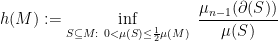
where the ${\partial (S)}$ is the boundary of ${S}$ , ${\mu}$ is the ${n}$ -dimensional measure, and ${\mu_{n-1}}$ is ${(n-1)}$ -th dimensional measure defined using ${g}$ . Then

$\displaystyle h(M) \leq 2 \sqrt{\lambda_2} \ \ \ \ \ (1)$

The purpose of this post is to describe to the reader who knows nothing about differential geometry and who does not remember much multivariate calculus (that is, the reader who is in the position I was in a few weeks ago) what the above statement means, to describe the proof, and to see that it is in fact the same proof as the proof of the statement about graphs.

In this post we will define the terms appearing in the above theorem, and see their relation with analogous notions in graphs. In the next post we will see the proof.

First we recall the definitions in the case of graphs, which are good “models” to keep in mind as we will give the definitions of a manifold and of the Laplacian of a manifold.

Let ${G=(V,E)}$ be a ${d}$ -regular graph and ${A}$ be the adjacency matrix of ${G}$ . If ${S\subseteq V}$ is a subset of vertices, its volume ${\mu(S)}$ is defined as the sum of the degrees of the elements of ${S}$ , ${\mu(S):= d|S|}$ . The boundary ${\partial (S)}$ of ${S}$ is the set of edges that have one endpoint in ${S}$ and one endpoint in ${V-S}$ ; the conductance of ${S}$ is

$\displaystyle \phi(S):= \frac{|\partial(S)|}{\mu(S)}$

and the conductance of ${G}$ is defined as

$\displaystyle \phi(G):= \min_{S\subseteq V: 0 < \mu(S) \leq \frac 12 \mu(V) } \phi(S)$

The Laplacian matrix of ${G}$ is defined as ${L:= I - \frac 1d A}$ , where ${A}$ is the adjacency matrix of ${G}$ . Since ${L}$ is a symmetric real matrix, all its eigenvalues are real, and, if we call them ${\lambda_1 \leq \lambda_2 \leq \cdots \leq \lambda_n}$ , the Cheeger inequality in graphs is

$\displaystyle \frac {\lambda_2} 2 \leq \phi(G) \leq \sqrt{2 \lambda_2} \ \ \ \ \ (2)$

1. Manifolds, gradient, and divergence

1.1. What is a manifold?

First let us discuss (non-rigorously) what is a manifold: we can think of an ${n}$ -dimensional manifold as a subset ${M \subseteq {\mathbb R}^m}$ , for some ${m}$ , such that for every point ${x\in M}$ , if we look at a small ball around ${x}$ , the intersection of the ball with ${M}$ looks like a ball in ${{\mathbb R}^n}$ . For example, consider a two-dimensional sphere in ${{\mathbb R}^2}$ : for every point on the sphere, a small neighborhood around it looks like a flat disc.

The formalization of this notion, which will turn out not to require us to think of ${M}$ as a subset of ${{\mathbb R}^m}$ is rather technical, and it has quite a lot of pieces. Instead of introducing the rigorous definition piece by piece, and trying to understand what a manifold is, I think it’s better to start by thinking about what a manifold does, that is, what kind of properties we want from the definition, and what kind of calculations we want the definition to allow, and then the details of the definition is just whatever works to capture these intentions.

Basically, we would like to be able to do with an ${n}$ -dimensional manifold ${M}$ most of the things we would do with ${{\mathbb R}^n}$ . We would like to have a distance function ${dist(x,y)}$ between elements ${x,y \in M}$ that satisfies the triangle inequality and that is the “length of the shortest path” from ${x}$ to ${y}$ in ${M}$ , we would like to have a measure ${\mu}$ , that gives us the “volume” ${\mu(A)}$ of a subset ${A\subseteq M}$ . If we define functions ${f: M \rightarrow {\mathbb R}}$ , we would like to integrate them, and compute ${\int_M f {\rm d} \mu}$ , or ${\int_A f {\rm d} \mu}$ , where ${A\subseteq M}$ . We would also like to have a definition of continuous functions ${f: M \rightarrow {\mathbb R}}$ , or ${f:M \rightarrow {\mathbb C}}$ , or ${f:M \rightarrow {\mathbb R}^k}$ , and, finally, we would like to define derivatives of functions ${f: M \rightarrow {\mathbb R}}$ .

On the other hand, we will not try to think of the elements of ${M}$ as vectors, and, in particular, we will not have a definition of adding elements of ${M}$ , or multiplying them by constants, much less of taking an inner product of them. (This means that the distance function will not come from a norm.) To see why not, consider a 2-dimensional sphere in ${{\mathbb R}^3}$ . We want to think of it as completely symmetric under rotations, so there can be no meaningful notion of a point on the sphere being “bigger” than another, so if ${x}$ is a point on the sphere, there isn’t a meaningful notion of ${2\cdot x}$ . (You could try to say ${2\cdot x = x}$ , but then this would imply ${x=0}$ .)

Because a manifold is not a vector space, it is tricky to define derivatives. We want to think of an ${n}$ -dimensional manifold as a generalization of ${{\mathbb R}^n}$ , and a function ${f:{\mathbb R}^n \rightarrow {\mathbb R}}$ does not have a derivative. Instead, for every direction ${y}$ , it has a partial derivative at ${x}$ in the direction ${y}$

$\displaystyle \frac{\partial f}{\partial y} (x) = \lim_{\epsilon \rightarrow 0} \frac {f(x+\epsilon y) - f(x)}{\epsilon}$

and the above expression requires us to add elements of ${{\mathbb R}^n}$ and to multiply them by constants.

However, if we look at a point ${x}$ , the immediate neighborhood of ${x}$ does look like a small piece of ${{\mathbb R}^n}$ , which is a vector space. To make this intuition formal, instead of trying to formalize the notion of “small piece of a vector space,” one defines directional derivatives where the direction ${y}$ is not in ${M}$ but in the tangent space to ${M}$ at ${x}$ , which is a honest-to-God vector space.

In the rigorous definition, we have a topology on ${M}$ , which allows to talk about “small intervals around” a point ${x}$ , and to talk about “continuous functions” ${f: M \rightarrow X}$ where ${X}$ can be ${{\mathbb R}}$ , ${{\mathbb C}}$ , ${{\mathbb R}^k}$ , and so on. Then, for every small interval around a point ${x}$ we have an ${n}$ -dimensional coordinate system, which we can think of as an approximation of the interval around ${x}$ as a piece of ${{\mathbb R}^n}$ ; these coordinate systems are called “charts” and their collection is called an “atlas.” Charts of nearby points are supposed to be “consistent in their intersection,” which is assured by consistent mappings between them. For every point ${x}$ we also have an ${n}$ -dimensional vector space, which is the tangent space at ${x}$ . There are also mapping that relate the tangent spaces of nearby points. Finally, we have a “metric,” that, to make things more confusing, is not a distance function that satisfies the triangle inequality, but is the definition of an inner product between vectors of the tangent spaces. From the metric, it is possible to define a distance function on ${M}$ that satisfies the triangle inequality, and a measure ${\mu}$ , and from the measure we can define integrals. Taking partial derivatives is still a bit tricky, and we will return to it when we talk about the gradient.

If ${S\subseteq M}$ is a subset of the manifold, then the boundary ${\partial S}$ of ${S}$ is the set of points ${x}$ such that there are arbitrarily small intervals around ${x}$ that contain both elements of ${S}$ and elements of ${M-S}$ . For nice enough ${S}$ , ${\partial S}$ will be an ${(n-1)}$ -dimensional object, so we will have ${\mu(S)=0}$ , but we can use the metric to define an ${(n-1)}$ -dimensional measure ${\mu_{n-1}}$ .

So we have a general sense of the definition of the Cheeger constant in manifold. For the analogy to graphs, we should think of the points of ${M}$ as ${V}$ , of ${\mu(S)}$ as ${d|S|}$ , of infinitesimally close points ${x,y}$ as an edge, and of the boundary ${\partial S}$ of a set as the set of edges leaving ${S}$ .

1.2. What is the Laplacian?

Now we have to define the Laplacian. The Laplacian is a linear operator that maps a function ${f: M \rightarrow {\mathbb R}}$ to a function ${Lf : M \rightarrow {\mathbb R}}$ , and it is defined as

$\displaystyle Lf := - {\rm div} \nabla f$

where ${\nabla}$ is the gradient operator and ${{\rm div}}$ is the divergence operator. (All the functions that we talk about are infinitely differentiable.)

To see what these operators are, and what they have to do with the Laplacian of graphs, recall that, in a graph,

$\displaystyle (Lf)_v = f_v - \frac 1d \sum_{w: (v,w)\in E} f_w$

the Laplacian of ${f\in {\mathbb R}^V}$ at ${v}$ is the difference between the value of ${f}$ at ${v}$ and the average value of ${f}$ at neighbors of ${v}$ . Similarly, in a manifold, ${(Lf)(x)}$ measures how much bigger ${f(y)}$ tends to be on average than ${f(x)}$ at a random point ${y}$ close to ${x}$ .

We will give some intuition about how the definition of the Laplacian in ${{\mathbb R}^n}$ matches the intuition from the case of graphs. The generalization from ${{\mathbb R}^n}$ to an ${n}$ -dimensional manifold is quite technical, but the general intuition is similar.

1.3. The Laplacian in one dimension

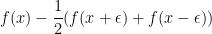
To see how to formalize this intuition, suppose ${M={\mathbb R}}$ and so ${f: {\mathbb R} \rightarrow {\mathbb R}}$ . Then, our intuition for the Laplacian of ${f}$ at ${L}$ is that, for a small ${\epsilon}$ , we should look at

$\displaystyle f(x) - \frac 12 (f(x+\epsilon) + f(x-\epsilon))$

Qualitatively, this quantity is positive if ${f}$ is concave and negative if ${f}$ is convex, so it seems related to ${-f''(x)}$ , where ${f''}$ is the second derivative of ${f}$ . Indeed, the Taylor expansion of ${f}$ at ${x}$ is

$\displaystyle f(x+\epsilon) \approx f(x) + \epsilon f'(x) + \frac {\epsilon^2}2 f''(x)$

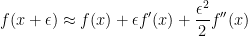
and so

$\displaystyle f(x) - \frac 12 (f(x+\epsilon) + f(x-\epsilon)) \approx -\frac 12 \epsilon^2 f''(x)$

And, indeed, for functions ${f: {\mathbb R} \rightarrow {\mathbb R}}$ both the gradient operator and the divergence operator are just the derivative operator, and so 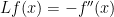${Lf(x) = -f''(x)}$ and we have

$\displaystyle Lf(x) = \lim_{\epsilon \rightarrow \infty} \frac 1{\epsilon^2} \cdot (2f(x) - f(x+\epsilon) -f(x-\epsilon))$

which matches our intuition from the case of graphs.

For functions ${f: {\mathbb R} \rightarrow {\mathbb R}}$ , the operator ${L}$ is linear, and we may ask if it has eigenvalues and eigenfunctions, that is, if there are numbers ${\lambda}$ and functions ${f}$ for which the equation

$\displaystyle Lf = \lambda f$

holds. Let’s see: what functions are equal to their second derivative, up to a multiplicative constant? For example, ${\sin kx}$ and ${\cos kx}$ are, where ${k}$ is an integer. (So is ${e^{kx}}$ .)

Now suppose that our manifold ${M}$ is a unit circle in the plane, that is, points of ${M}$ are of the form ${(\sin x,\cos x)}$ . This is a (one-dimensional) manifold because a small arc around a point is quite close to being a straight segment. If ${f: {\mathbb R} \rightarrow {\mathbb R}}$ is periodic with period ${[0,2\pi]}$ , we can use it to define a function ${F}$ on ${M}$ , where ${F(\sin x, \cos x) = f(x)}$ ; similarly, if ${F:M \rightarrow {\mathbb R}}$ is defined on the circle we can think of it as a periodic function ${f}$ with period 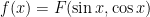${[0,2\pi]}$ , where ${f(x) = F(\sin x,\cos x)}$ . In fact, there isn’t really any difference between thinking of functions defined over ${M}$ and periodic functions of period ${[0,2\pi]}$ , and the Laplacian of ${M}$ will be the operator that takes a periodic function to minus its second derivative. So ${\sin kx}$ and ${\cos kx}$ will be eigenvectors of the Laplacian of the circle, with eigenvalues ${\approx k^2}$ . Note the extreme similarity to the spectrum of the circle as a graph, where the eigenvectors are vectors whose ${j}$ -th coordinate is ${\sin 2\pi kj/n}$ or ${\cos 2\pi k j/n}$ and ${2\pi j/n}$ ranges in ${[0,2\pi]}$ . The main difference is one of normalization: in the circle graph, all eigenvalues are at most 2, at the smallest positive one is about ${1/n^2}$ ; in the circle manifold the eigenvalues are arbitrarily large, and the smallest positive one is 1. However, if we call ${\lambda_k}$ the ${k}$ -th smallest eigenvalue, in both cases we have that ${\lambda_k/\lambda_2}$ is about ${k^2}$ .

1.4. The gradient in ${{\mathbb R}^n}$

For the higher-dimensional case, let us start from the case ${M={\mathbb R}^n}$ . In this case, let us fix the orthonormal basis ${{\bf e}_1,\ldots,{\bf e}_n}$ for ${{\mathbb R}^n}$ where ${{\bf e}_i}$ is the vector that has zeroes everywhere except a 1 in the ${i}$ -th position. For a function ${f: {\mathbb R}^n \rightarrow {\mathbb R}}$ , its gradient ${\nabla f}$ is a function that maps a point ${{\bf x}}$ to an ${n}$ -dimensional vector, which contains the partial derivatives of ${f}$ , that is

$\displaystyle \nabla f ({\bf x}) = \left( \frac {\partial f}{\partial {\bf e}_1}({\bf x}),\ldots,\frac{\partial f}{\partial {\bf e}_n}({\bf x})\right)$

where, for a vector ${{\bf y}}$ , the partial derivative ${\frac {\partial f}{\partial {\bf y}} }$ is the function

$\displaystyle \frac {\partial f}{\partial {\bf y}} ({\bf x}) = \lim_{\epsilon \rightarrow 0} \frac{f({\bf x}+\epsilon {\bf y}) - f({\bf x})}{\epsilon}$

If ${{\bf y}}$ and ${{\bf z}}$ are orthogonal then

$\displaystyle \frac {\partial f}{\partial {\bf y}+{\bf z}} (x) = \frac {\partial f}{\partial {\bf y}} ({\bf x}) + \frac {\partial f}{\partial {\bf z}} ({\bf x})$

this means that for every vector ${{\bf y}=(y_1,\ldots,y_n)}$ we have

$\displaystyle \frac {\partial f}{\partial {\bf y}} ({\bf x}) = \sum_i \frac {\partial f}{\partial {\bf e}_i} ({\bf x}) \cdot y_i = \langle \nabla f({\bf x}), {\bf y}\rangle$

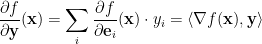
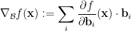
It is important to note that there was nothing special about the use of the base ${\{ {\bf e}_1,\ldots,{\bf e}_n\}}$ . Take an arbitrary orthonormal base ${{\cal B} := \{ {\bf b}_1,\ldots,{\bf b}_n \}}$ , then define the “base- ${\cal B}$ ” gradient as

$\displaystyle \nabla_{\cal B} f({\bf x}):= \sum_i \frac{\partial f}{\partial {\bf b}_i}({\bf x}) \cdot {\bf b}_i$

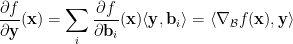
then we again have that for every ${{\bf y}}$ , after writing ${{\bf y} = \sum_i \langle {\bf y},{\bf b}_i\rangle \cdot {\bf b}_i}$ ,

$\displaystyle \frac {\partial f}{\partial {\bf y}} ({\bf x}) = \sum_i \frac {\partial f}{\partial {\bf b}_i} ({\bf x}) \langle {\bf y},{\bf b}_i\rangle = \langle \nabla_{\cal B} f({\bf x}) ,{\bf y} \rangle$

so, in fact, ${\nabla_{\cal B} f({\bf x})}$ is always the same vector ${\nabla f({\bf x})}$ regardless of the choice of ${\cal B}$ .

Indeed, we could take as the definition of the gradient to say that ${\nabla f({\bf x})}$ is the unique vector that satisfies the equation

$\displaystyle \frac {\partial f}{\partial {\bf y}} ({\bf x}) = \langle \nabla f({\bf x}), {\bf y} \rangle$

for every ${{\bf y}}$ .

It is also worth nothing that, among all unit vectors ${{\bf y}}$ , the one that maximizes ${\frac {\partial f}{\partial {\bf y}} ({\bf x})}$ is the one parallel to ${\nabla f({\bf x})}$ , so ${\nabla f({\bf x})}$ points in the direction in which ${f}$ grows the most near ${f}$ , which is the most intuitive interpretation.

If ${f: M \rightarrow {\mathbb R}}$ in general, then ${\nabla f(x)}$ is a vector in the tangent space of ${M}$ at ${x}$ , and the directional derivative ${\frac{\partial f}{\partial y}(x)}$ , where ${y}$ is a vector in the tangent space at ${x}$ , satisfies

$\displaystyle \frac{\partial f}{\partial y}(x) = \langle \nabla f(x), y \rangle$

where the inner product is in the tangent space. The definition of partial derivative, and the fact that there is a vector ${\nabla f(x)}$ that satisfies the above equation for every ${y}$ is beyond the scope of these notes.

1.5. The divergence in ${{\mathbb R}^n}$

The definition of divergence is a bit more tricky. If ${M ={\mathbb R}^n}$ , then ${{\rm div}}$ takes in input a function ${g: {\mathbb R}^n \rightarrow {\mathbb R}^n}$ , and returns a function ${{\rm div} g : {\mathbb R}^n \rightarrow {\mathbb R}}$ . The definition of ${{\rm div} g({\bf x})}$ , (up to scaling) can be thought of as follows: consider a small sphere of radius ${\epsilon}$ around ${{\bf x}}$ , pick a random element of the sphere by picking a random unit vector ${{\bf y}}$ and considering the vector ${{\bf x}+\epsilon {\bf y}}$ , and then look at the average value of

$\displaystyle \frac 1 \epsilon \langle g({\bf x}+\epsilon {\bf y}), {\bf y}\rangle$

which is the component of ${g({\bf x}+\epsilon {\bf y})}$ that “points away” from ${{\bf x}}$ in the direction of the line that joins ${{\bf x}}$ to ${{\bf x} + \epsilon {\bf y}}$ .

This will be positive if the vector ${g({\bf y})}$ tends to point away from ${{\bf x}}$ , for random ${{\bf y}}$ close to ${{\bf x}}$ , and negative otherwise.

1.6. The Laplacian in ${{\mathbb R}^n}$

Now let us see what happens when we instantiate this definition to ${g({\bf x}) = \nabla f({\bf x})}$ . We pick a random unit vector ${y}$ , and we compute

$\displaystyle \frac 1\epsilon \langle \nabla f({\bf x}+\epsilon {\bf y}), {\bf y} \rangle = \frac 1 \epsilon \cdot \frac {\partial f}{\partial {\bf y}} ({\bf x}+\epsilon {\bf y})$

For small ${\epsilon}$ ,

$\displaystyle \frac {\partial f}{\partial {\bf y}} ({\bf x}+\epsilon {\bf y}) \approx \frac{ f({\bf x}+ 2\epsilon {\bf y}) - f({\bf x}+\epsilon {\bf y}) }{\epsilon}$

$\displaystyle {\rm div} \nabla f({\bf x}) \approx \frac 1 {\epsilon^2} \mathop{\mathbb E}_{{\bf y} \in S_{n-1}} f({\bf x}+2\epsilon {\bf y}) - f({\bf x}+\epsilon {\bf y})$

which is the average rate of growth of ${f}$ in a random direction. So we have that 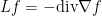${Lf = - {\rm div} \nabla f}$ is the rate of decrease of ${f}$ in a random direction. This is roughly the equivalent of the discrete case where ${Lf_v}$ is the difference between ${f_v}$ and the average value of ${f_w}$ for a random neighbor ${w}$ of ${v}$ .

It turns out that we can also make the correspondence between the discrete and the continuous case closer, by finding linear operators in the discrete case whose composition gives the Laplacian, and that are somewhat analogous to ${\nabla}$ and ${- {\rm div}}$ .

Consider the ${|E| \times n}$ incidence matrix ${C}$ of ${G}$ defined as follows:

$\displaystyle C_{uv,w} = \left\{ \begin{array}{cl} 1 & \mbox{ if } (u,v)\in E \wedge u=w\\ -1 & \mbox{ if } (u,v)\in E \wedge v=w\\ 0 & \mbox{ otherwise} \end{array} \right.$

where we have fixed an arbitrary orientation of the edges of ${E}$ . Then ${Cf}$ is an ${|E|}$ -dimensional vector such that ${Cf_{uv}}$ equals ${f_u-f_v}$ for every (directed) edge ${(u,v) \in E}$ . We can also think of ${Cf}$ as mapping a vertex ${u}$ to a ${degree(u)}$ -dimensional vector ${Cf_{u,*}}$ , whose ${i}$ -th coordinate is ${f_u - f_v}$ where ${(u,v)}$ is the ${i}$ -th outgoing edge from ${u}$ . In this view, ${C}$ acts somewhat like the ${- \nabla}$ , giving us all the “derivatives” of ${f_u}$ in all directions. (The minus sign is because in the derivative at ${x}$ we consider ${f(y)-f(x)}$ where ${y}$ is close to ${x}$ , but ${Cf_{u,*}}$ “at ${v}$ ” gives us ${f_u-f_v}$ .)

If ${g}$ is an ${|E|}$ -dimensional vector, then

$\displaystyle C^T g_v = \sum_{w: (v,w)\in E} g_{v,w} - \sum_{u: (u,v) \in E} g_{u,v}$

is the flow through ${v}$ , if we think of ${g}$ as defining a flow on the (directed) edges of ${G}$ . This is the analog of the divergence ${{\rm div} g(x)}$ , which also computes the net flow of ${g}$ away from a point ${x}$ .

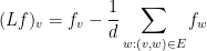
The reader can verify that we indeed have ${L= C^T C}$ .

3 thoughts on “The Cheeger inequality in manifolds”

diego on April 1, 2013 at 11:29 pm said:

Amazing post! (a small typo: there’s a limit with epsilon tending to infty instead of 0)
anon on December 16, 2019 at 12:49 pm said:

awesoem post, thanks
Pingback: Buser Inequalities in Graphs | in theory

in theory

"Marge, I agree with you – in theory. In theory, communism works. In theory." — Homer Simpson

The Cheeger inequality in manifolds

3 thoughts on “The Cheeger inequality in manifolds”

Leave a comment

Share this:

Related

3 thoughts on “The Cheeger inequality in manifolds”

Leave a comment