Decomposition Results and Regularity Lemmas

Several results in additive combinatorics have the flavor of decomposition results in which one shows that an arbitrary combinatorial object can be approximated by a “sum” of a “low complexity” part and a “pseudorandom” part. This is helpful because it reduces the task of proving that an arbitrary object has a certain property to the easier task of proving that low-complexity objects and pseudorandom objects have the property. (Provided that the property is preserved by the approximation and the sum.)

Many examples of such results are given in the paper accompanying Terry Tao’s tutorial at FOCS’07.

Usually, one needs a strong notion of approximation, and in such cases the complexity of the “low complexity” part is fantastically large (a tower of exponentials in the approximation parameter), as in the Szemeredi Regularity Lemma, which can be seen as a prototypical such “decomposition” result. In some cases, however, weaker notions of approximation are still useful, and one can have more reasonable complexity parameters, as in the Weak Regularity Lemma of Frieze and Kannan.

A toy example of a “weak decomposition result” is the following observation: let $\chi_r: \{0,1\}^n \rightarrow \{ -1,1\}$ be the linear functions $\chi_r (x) := (-1)^{\sum_i r_i x_i }$ used as the basis for Fourier analysis of functions $f: {\mathbb F}_2^n \rightarrow {\mathbb R}$ , let $g: {\mathbb F}_2^n \rightarrow [-1,1]$ be a bounded function, and consider its Fourier transform

$\displaystyle g(x) = \sum_r \hat g(r) \chi_r (x)$

Then we can write

$g = h_1 + h_2$

where

$h_1(x) := \sum_{r : |\hat g(r)| \geq \epsilon } \hat g(r) \chi_r (x)$

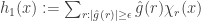
is the truncation of the Fourier expansion containing only the larger coefficient, and $h_2 := g-h_1$ . Since we know 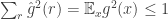$\sum_r \hat g^2 (r) = {\mathbb E}_x g^2(x) \leq 1$ , we can see that $h_1$ is defined as a linear combination of at most $1/\epsilon^2$ functions $\chi_r$ , and so it has “low complexity” relative to the linear functions.

The other observation is that, for every function $\chi_r$ , we have

$\displaystyle | {\mathbb E}_x h_2 (x) \chi_r (x) | = | \hat h_2 (r) | \leq \epsilon$

So we have written $g$ as a sum of a function of “complexity” $O(1/\epsilon^2)$ and of a “pseudorandom” function all whose Fourier coefficients are small. The reason we think of a function with small Fourier coefficients as “pseudorandom” is because (the uniform distribution over) a set is $\epsilon$ -biased (in the Naor-Naor sense) if and only if its indicator function has small Fourier coefficients. Another way to look at the decomposition is to see that we have found a function $h_1$ that has “small complexity” relative to the set of Fourier basis functions $\chi_r$ , and such that $h_1$ and $g$ are indistinguishable by basis functions, that is,

$| {\mathbb E}_x g(x)\chi_r (x) - {\mathbb E}_x h_1(x) \chi_r (x) | \leq \epsilon$

These are trivial observation, and they seem to depend essentially on the fact that the $\chi_r$ are orthogonal. Indeed, this is not the case.

By modifying the main idea in the Frieze-Kannan paper, it is possible to prove the following result.

Theorem 1 (Low Complexity Approximation, Simple Version) Let $(X,\mu)$ be a probability space, $g:X \rightarrow [-1,1]$ a bounded function, $F$ a collection of bounded functions $f:X \rightarrow [-1,1]$ , and $\epsilon$ an approximation parameter.

Then there is a function $h: X \rightarrow {\mathbb R}$ such that

$h$ has low complexity relative to $F$ :
$h:= \sum_{i=1}^k c_i f_i$

where $k\leq \epsilon^{-2}$ , $f_i\in F$ , and the coefficients $c_i$ satisfy $\sum_{i=1}^k c_i^2 \leq 1$ ;
$h$ is $\epsilon$ -indistinguishable from $g$ by $F$ :
$\forall f\in F. \ \ | {\mathbb E}_{x \sim \mu} f(x) \cdot (g(x)-h(x)) | \leq \epsilon$

We can see that the Fourier analysis approximation we discussed above is the special case in which $F$ is the set of linear functions.

The proof is surprisingly simple. Assume without loss of generality that $F$ is “closed under negation,” that is, if $f\in F$ then $-f \in F$ . (Otherwise we apply the following argument to the closure of $F$ .) We construct the function $h$ via the following algorithm.

$h_0 :=$ 0; $t= 0$
while such that
- $h_{t+1} := h_t + \epsilon f_{t+1}$
- $t:=t+1$

If the algorithm terminates after a finite number $k$ of steps, then the function $h_k$ is indistinguishable as required, and we have $h_k = \sum_{i=1}^k \epsilon f_k$ , so we just need to argue that the algorithm always terminates, and it does so within $k\leq \epsilon^{-2}$ steps.

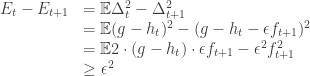
We prove this via an energy decreasing argument. Consider the error at time $t$ , $\Delta_t := g-h_t$ , and define the “energy” at time $t$ to be $E_t := {\mathbb E} \Delta_t^2$ . At time zero, $E_0 := {\mathbb E} g^2 \leq 1$ . It remains to show that the energy decreases by at least $\epsilon^2$ at every step. (The energy is always non-negative, so if it starts at 1 and it decreases by $\epsilon^2$ at least at every step, there can be no more than $\epsilon^{-2}$ steps.)

$\displaystyle \begin{array}{lll} E_{t} - E_{t+1} & = {\mathbb E} \Delta_{t}^2 - \Delta_{t+1}^2 \\ & = {\mathbb E} (g-h_t)^2 - (g-h_t-\epsilon f_{t+1})^2\\ & = {\mathbb E} 2 \cdot (g-h_t) \cdot \epsilon f_{t+1} - \epsilon^2 f_{t+1}^2\\ & \geq \epsilon^2 \end{array}$

To see how Theorem 1 relates to the regularity lemma on graphs, let $X$ be the set of edges in the complete graph $K_n$ over $n$ vertices, and let $G$ be an arbitrary graph over $n$ vertices, which we shall think of as a function $G:X \rightarrow \{ 0,1 \}$ . For two disjoint sets of vertices $S,T$ , let $f_{S,T} : X \rightarrow \{ 0,1\}$ be the indicator function of the set of edges with one endpoint in $S$ and one endpoint in $T$ , let $F$ be the set of such functions, and let $\mu$ be the uniform distribution over $X$ . Then, for every $\epsilon$ , Theorem 1 gives us an approximating weighted graph $H: X \rightarrow {\mathbb R}$ such that

$H$ is a weighted sum of $\leq \epsilon^{-2}$ functions $f_{S_i,T_i}$
For every two sets of vertices $S,T$ , the number of edges in $G$ between $S$ and $T$ differs from the (weighted) number of edges in $H$ between $S$ and $T$ by at most $\epsilon n^2$ . (Indeed, at most $\epsilon {n \choose 2}$ .)

The model graph $H$ is helpful because one can solve several optimization problems on it (such as Max Cut) in time dependent only on $\epsilon$ , and then transfer such solutions to $G$ , paying an additive cost of $\epsilon n^2$ (which is negligible if $G$ is dense).

Regularity Lemmas, however, are usually stated in terms of partitions of the sets of vertices, not in terms of linear combinations. Also, it is somewhat undesirable that the approximating graph $H$ has weights that are not guaranteed to be bounded. Analogously, in Theorem 1, it would be desirable for $h$ to be bounded, which is not guaranteed by the construction. (Although one can see that ${\mathbb E} h^2 = O(1)$ , the best bound we can give about individual inputs is $|h(x)| \leq \epsilon^{-1}$ .)

To deal with this issue, we first need a couple of definitions.

If $P = \{ B_1,\ldots,B_m \}$ is a partition of $X$ , and $g: X \rightarrow {\mathbb R}$ is any function, then the conditional expectation of $g$ on $P$ is the function $g_P : X \rightarrow {\mathbb R}$ defined as

$g_P (x) := {\mathbb E} [ g_P(y) | \ y\in B_i : x \in B_i ]$

that is, on input $x$ , belonging to block $B_i$ of the partition $P$ , the value of $g_P(x)$ is the expectation of $g$ on the block $B_i$ . To visualize this definition, suppose that elements of $X$ are people, $B_i$ are countries, and $g(x)$ is the wealth of person $x$ . Now, spread around the wealth evenly within each country; then $g_p(x)$ is the post-spreading-around wealth of $x$ .

The following definition will simplify some discussions on indistinguishability: if $(X,\mu)$ is a probability space, $F$ is a collection of functions $f: X \rightarrow {\mathbb R}$ and $g: X \rightarrow {\mathbb R}$ is any function, then

$(1) \ \ \ || g||_F := \sup_{f\in F} | {\mathbb E} fg |$

Note that this is indeed a norm, and that $g$ and $h$ are $\epsilon$ -indistinguishable by $F$ if and only if $|| g-h||_F \leq \epsilon$ .

Given these definitions, Frieze and Kannan prove that, in the special case in which $X$ are edges of a complete graph and $F$ is the collection of indicator functions of cuts, if $P$ is a partition of $X$ defined by first picking functions $f_1,\ldots,f_k \in F$ and then creating the coarsest partition such that every function $f_i$ is constant on each block of the partition (we call $P$ the partition generated by $f_1,\ldots,f_k$ ), and if $g:X \rightarrow [-1,1]$ is any function and $h: X \rightarrow {\mathbb R}$ is a function which is constant on each block of $f$ , then

$(2) \ \ \ || h - g_p ||_F \leq || h-g||_F$

From this, we have that if $h = \sum_i c_i f_i$ is the function of Theorem 1, and $P$ is the partition defined by the $f_i$ , then

$|| g- g_p||_F \leq || g-h||_F + || h-g_p||_F \leq 2 ||g-h||_F \leq 2\epsilon$

And so the function $g_p$ is also a good approximation for $g$ . Nicely, $g_p$ is precisely the type of approximation described in the standard regularity lemma, and all its edge weights are between 0 and 1. I don’t know how to prove (2) in general, but the iterative partitioning proof of the Weak Regularity Lemma can be abstracted into the following result.

Theorem 2 (Low Complexity Approximation, Partition Version) Let $(X,\mu)$ be a probability space, $g:X \rightarrow [-1,1]$ a bounded function, $F$ a collection of boolean functions $f:X \rightarrow \{ -1,1\}$ , and $\epsilon$ an approximation parameter.

Then there is a function $h: X \rightarrow [-1,1]$ such that

$h$ has low complexity relative to $F$ : there are $k= O( \epsilon^{-2})$ functions $f_i\in F$ such that $h := g_P$ , where $P$ is the partition generated by $f_1,\ldots,f_k$ ;
$h$ is $\epsilon$ -indistinguishable from $g$ by $F$ , that is,
$|| g-h||_F \leq \epsilon$

The proof proceeds by starting with $P$ being the trivial partition containing only one block; we continue until we have a partition $P$ such that $|| g-g_P||_F \leq \epsilon$ . If the current partition is such that $|| g-g_P||_F > \epsilon$ then we add the function $f$ such that $| {\mathbb E} f(g-g_P) | > \epsilon$ to the collection of functions used to define $g_p$ . Every time we thus refine $P$ , we can show that ${\mathbb E} g_P^2$ increases by $\Omega(\epsilon^2)$ , and it is always at most one, so we are able to bound the number of steps.

Note that, in Theorems 1 and 2, we do not need $X$ to be finite; indeed, $(X,\mu)$ can be any measure space such that $\mu(X)=1$ , provided we interpret the notation ${\mathbb E} f$ to mean $\int_X f d\mu$ . (In such cases, we shall also need to make proper integrability assumptions on $g$ and the functions in $f$ .) From Theorems 1 and 2 we can reconstruct the “Analytic Weak Regularity Lemmas” of Lovasz and Szegedy. For example, if $X = [0,1]^2$ , and $F$ is the class of functions of the form $1_{S\times S}$ , over all measurable sets $S$ , then the norm $|| \cdot ||_F$ is the same as the norm $|| \cdot ||_\Box$ defined in Section 4 of the Lovasz-Szegedy paper, and their Lemma 7 follows from our Theorem 1.

For a complexity-theoretic interpretation, note that, in Theorem 2, we can take $F$ to be the class of functions computable by circuits of size at most $S$ ; then the theorem gives us an approximating function $h$ which can be computed in size $S \cdot exp (O(\epsilon^{-2}))$ .

Could we make the complexity of the approximation polynomial in $1/\epsilon$ , while retaining the useful property that the approximating function is bounded? This is the subject of a new paper by Madhur Tulsiani, Salil Vadhan, and I, and also the subject of a forthcoming post.

3 thoughts on “Decomposition Results and Regularity Lemmas”

Pingback: Boosting and the Regularity Lemma « in theory
anonymous on December 9, 2008 at 10:40 pm said:

Why the complexity of $h$ is Theorem 2 is $S.exp(O(\epsilon ^{-2})$ ?
anonymous on December 9, 2008 at 10:41 pm said:

I don’t see a way other than going over all X and computing all f’s to find out the partition the input is in, and then computing f over all of that domain and taking the average 😦

in theory

"Marge, I agree with you – in theory. In theory, communism works. In theory." — Homer Simpson

Decomposition Results and Regularity Lemmas

3 thoughts on “Decomposition Results and Regularity Lemmas”

Leave a comment

Share this:

Related

3 thoughts on “Decomposition Results and Regularity Lemmas”

Leave a comment