Online Optimization Post 3: Follow the Regularized Leader

The multiplicative weights algorithm is simple to define and analyze, and it has several applications, but both its definition and its analysis seem to come out of nowhere. We mentioned that all the quantities arising in the algorithm and its analysis have statistical physics interpretations, but even this observation brings up more questions than it answers. The Gibbs distribution, for example, does put more weight on lower-energy states, and so it makes sense in an optimization setting, but to get good approximations one wants to use lower temperatures, while the distributions used by the multiplicative weights algorithms have temperature ${1/\epsilon}$ , where ${2\epsilon}$ is the final “amortized” regret bound, so that one uses, quite counterintuitively, higher temperatures for better approximations.

Furthermore, it is not clear how we would generalize the ideas of multiplicative weights to the case in which the set of feasible solutions ${K}$ is anything other than the set of distributions.

Today we discuss the “Follow the Regularized Leader” method, which provides a framework to design and analyze online algorithms in a versatile and well-motivated way. We will then see how we can “discover” the definition and analysis of multiplicative weights, and how to “discover” another online algorithm which can be seen as a generalization of projected gradient descent (that is, one can derive the projected gradient descent algorithm and its analysis from this other online algorithm).

1. Follow The Regularized Leader

We will first state some results in full generality, making no assumptions on the set ${K}$ of feasible solutions or on the set of loss functions ${f_t : K \rightarrow {\mathbb R}}$ encountered by the algorithm at each step.

Let us try to define an online optimization algorithm from scratch. The solution ${x_t}$ proposed by the algorithm at time ${t}$ can only depend on the previous cost functions ${f_1,\ldots,f_{t-1}}$ ; how should it depend on it? If the offline optimal solution ${x}$ is consistently better than all others at each time step, then we would like ${x_t}$ to be that solution, so we want ${x_t}$ to be a solution that would have worked well in the previous steps. The most extreme way of implementing this idea is the Follow the Leader algorithm (abbreviated FTL), in which we set the solution at time ${t}$

$\displaystyle x_t := \arg\min_{x\in K} \sum_{k=1}^{t-1} f_k(x)$

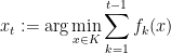
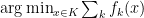
to be the best solution for the previous steps. (Note that the algorithm does not prescribe what solution to use at step ${t=1}$ .)

It is possible for FTL to perform very badly. Consider for example the “experts” setting in which we analyzed multiplicative weights: the set of feasible solutions ${K}$ is the set ${\Delta}$ of probability distributions over ${\{1,\ldots,n\}}$ , and the cost functions are linear ${f_t(x) = \sum_i \ell_t(i) x(i)}$ with coefficients ${0\leq \ell_t(i) \leq 1}$ . Suppose that ${n=2}$ and that ${x_1 = (0.5,.0.5)}$ . Then a possible run of the algorithm could be:

${x_1 = (.5,.5)}$ , ${\ell_1 = (0,.5)}$
${x_2 = (1,0)}$ , ${\ell_2 = (1,0)}$
${x_3 = (0,1)}$ , ${\ell_3 = (0,1)}$
${x_4 = (1,0)}$ , ${\ell_4 = (1,0)}$
${x_5 = (0,1)}$ , ${\ell_5 = (0,1)}$

$\displaystyle \vdots$

In which, after ${T}$ steps, the algorithm suffers a loss of ${T- O(1)}$ while the offline optimum is ${T/2 + O(1)}$ . Thus, the regret is about ${T/2}$ , which compares very unfavorably to the ${O(\sqrt T)}$ regret of the multiplicative weight algorithm. For general ${n}$ , a similar example shows that the regret of FTL can be as high as about ${T\cdot \left( 1- \frac 1n \right)}$ .

In the above bad example, the algorithm keeps “overfitting” to the past history: if an expert is a bit better than the others, the algorithm puts all its probability mass on that expert, and the algorithm keeps changing its mind at every step. Interestingly, this is the only failure mode of the algorithm.

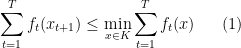
Theorem 1 (Analysis of FTL) For any sequence of cost functions ${f_1,\ldots,f_t}$ and any number of time steps ${T}$ , the FTL algorithm satisfies the regret bound

$\displaystyle {\rm Regret}_T \leq \sum_{t=1}^T f_t(x_t ) - f_t(x_{t+1} )$

So that if the functions ${f_t(\cdot)}$ are Lipschitz with respect to a distance function on ${K}$ , then the only way for the regret to be large is for ${x_t}$ to typically be far, in that distance, from ${x_{t+1}}$ .

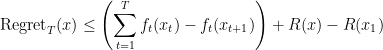
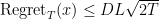
Proof: Recalling the definition of regret,

$\displaystyle {\rm Regret}_T := \sum_{t=1}^T f_t(x_t) - \min_{x\in K} \sum_{t=1}^T f_t(x) \ ,$

the theorem is equivalent to

$\displaystyle \sum_{t=1}^T f_t (x_{t+1}) \leq \min_{x\in K} \sum_{t=1}^T f_t(x) \ \ \ \ \ (1)$

We will prove (1) by induction. The base case ${T=1}$ is just the definition of ${x_2}$ . Assuming that $latex {(1)}&fg=000000$ is true up to ${T}$ we have

$\displaystyle \sum_{t=1}^{T+1} f_t (x_{t+1}) = \left( \sum_{t=1}^{T} f_t (x_{t+1}) \right) + f_{T+1} (x_{T+2}) \leq \sum_{t=1}^{T+1} f_t (x_{T+2}) = \min_{x\in K} \sum_{t=1}^{T+1} f_t(x)$

where the middle step follows from the use of the inductive assumption, which gives

$\displaystyle \sum_{t=1}^{T} f_t (x_{t+1}) \leq \min_{x\in K} \sum_{t=1}^T f_t (x) \leq \sum_{t=1}^T f_t (x_{T+2})$

$\Box$

The above example and analysis suggest that we should modify FTL in such a way that the choices of the algorithm don’t change too much from step to step, and that the solution ${x_t}$ at time ${t}$ should be a compromise between optimizing with respect to previous cost functions and not changing too much from step to step.

In order to do this, we introduce a new function ${R(\cdot)}$ , called a regularizer (more on it later), and, at each step, we compute the solution

$\displaystyle x_t := \arg\min_{x\in K} \ R(x) + \sum_{k=1}^{t-1} f_k(x)$

This algorithm is called Follow the Regularized Leader or FTRL. Typically, the function ${R(\cdot)}$ is chosen to be strictly convex and to take values that are rather big in magnitude. Then ${x_1}$ will be the unique minimum of ${R(\cdot)}$ and, at each subsequent step, ${x_t}$ will be selected in a way to balance the pull toward the minimum of ${R(\cdot)}$ and the pull toward the FTL solution ${\arg\min_{x\in K} \sum_k f_k(x)}$ . In particular, if ${R(\cdot)}$ is large in magnitude compared to each ${f_t(\cdot)}$ , the solution will not change too much from step to step.

We have the following analysis that makes no assumptions on ${K}$ , on the cost functions ${f_t(\cdot)}$ and on the regularizer (not even that the regularizer is convex).

Theorem 2 (Analysis of FTRL) For every sequence of cost functions and every regularizer function, the regret after ${T}$ steps of the FTRL algorithm is bounded as follows: for every ${x}$ ,

$\displaystyle {\rm Regret}_T(x) \leq \left( \sum_{t=1}^T f_t(x_{t}) - f_t (x_{t+1}) \right) + R(x) - R(x_1)$

where

$\displaystyle {\rm Regret}_T (x) := \sum_{t=1}^T f_t (x_t) - f_t (x)$

Proof: Let us run for ${T}$ steps the FTRL algorithm with regularizer ${R(\cdot)}$ and cost functions ${f_1,\ldots,f_T}$ , and call ${x_1,\ldots,x_T}$ the solutions computed by the FTL algorithm.

Now consider the following mental experiment: we run the FTL algorithm for ${T+1}$ steps, with the sequence of cost functions ${R,f_1,\ldots,f_t}$ , and we use ${x_1}$ as a first solution. Then we see that the solutions computed by the FTL algorithm will be precisely ${x_1,x_1,x_2,\ldots,x_T}$ . The regret bound for FTL implies that, for every ${x}$ ,

$\displaystyle R(x_1) - R(x) + \sum_{t=1}^T f_t(x_t) - f_t(x) \leq R(x_1) - R(x_1) + \sum_{t=1}^T f_t(x_t) - f_{t} (x_{t+1})$

$\Box$

Having established these results, the general recipe to solve an online optimization problem will be to find a regularizer function ${R}$ such that the minimum of ${R}$ “pulls away from” solutions that would make the FTL algorithm overfit, and such that there is a good balance between how big ${R}$ gets over ${K}$ (because we pay ${R(x^*) - R(x_1)}$ in the regret, where ${x^*}$ is the offline optimum) and how stable is the minimum of ${R(x) + \sum_{k=1}^{t-1} f_k(x)}$ as ${t}$ varies.

2. Negative-Entropy Regularization

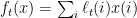
Let us consider again the “experts” setting, that is, the online optimization setup in which ${K}$ is the set of probability distributions over ${\{ 1,\ldots, n\}}$ and the cost functions are linear ${f_t (x) = \sum_i \ell_t (i) x(i)}$ with bounded coefficients.

The example we showed above showed that FTL will tend to put all the probability mass on one expert. We would like to choose a regularizer that fights this tendency by penalizing “concentrated” distributions and favoring “spread-out” distributions. This observation might trigger the thought that the entropy of a distribution is a good measure of how concentrated or spread out it is, although the entropy is actually higher for spread-out distribution and smaller for concentrated ones. So we will use as a regularizer minus the entropy, multiplied by an appropriate scaling factor:

$\displaystyle R(x) := c \cdot \sum_{i=1}^n x_i \ln x_i$

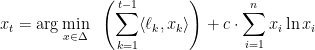
(Entropy is usually defined using logarithms in base 2, but using natural logarithms will make it cleaner to take derivatives, and it only affects the constant factor ${c}$ .) With this choice of regularizer, we have

$\displaystyle x_t = \arg\min_{x\in \Delta} \ \ \left( \sum_{k=1}^{t-1} \langle \ell_k , x_k \rangle \right ) + c \cdot \sum_{i=1}^n x_i \ln x_i$

To compute the minimum of the above function we will use the method of Lagrange multipliers. Specialized to our setting, the method of Lagrange multiplier states that if we want to solve the constrained minimization problem

$\displaystyle \min_{x : \ a^Tx = b } \ \ f(x )$

we introduce a new parameter ${\lambda}$ and define the function

$\displaystyle f_\lambda (x) := f(x) + \lambda \cdot (a^T x - b )$

Then it is possible to prove that if ${x^*}$ is a feasible minimizer of ${f(\cdot)}$ , then there is at least a value of ${\lambda}$ such that ${\nabla f_\lambda (x^*) = 0}$ , that is, such that ${x^*}$ is a stable point of ${f_\lambda}$ . So one can proceed by finding all ${x,\lambda}$ such that ${\nabla f_\lambda (x) = 0}$ and then filtering out the values of ${x}$ such that ${a^T x \neq b}$ , and finally looking at which of the remaining ${x}$ minimizes ${f(\cdot)}$ .

Ignoring for a moment the non-negativity constraints, the constraint ${x\in \Delta}$ reduces to ${\sum_i x_i = 1}$ , so we have to consider the function

$\displaystyle \left( \sum_{k=1}^{t-1} \langle \ell_k , x_k \rangle \right ) + c \cdot \left( \sum_{i=1}^n x_i \ln x_i \right) + \lambda \cdot \left( \langle x, {\bf 1} \rangle - 1\right)$

The partial derivative of the above expression with respect to ${x_i}$ is

$\displaystyle \left( \sum_{k=1}^{t-1} \ell_k (i) \right ) + c \cdot \left( 1 + \ln x_i \right) + \lambda$

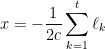
If we want the gradient to be zero then we want all the above expressions to be zero, which translates to

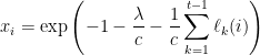
$\displaystyle x_i = {\rm exp} \left( -1 - \frac \lambda c - \frac 1c \sum_{k=1}^{t-1} \ell_k(i) \right)$

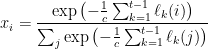
There is only one value of ${\lambda}$ that makes the above solution a probability distribution, and the corresponding solution is

$\displaystyle x_i = \frac {{\rm exp} \left( - \frac 1c \sum_{k=1}^{t-1} \ell_k(i) \right) } {\sum_j {\rm exp} \left( - \frac 1c \sum_{k=1}^{t-1} \ell_k(j) \right) }$

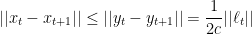
Notice that this is exactly the solution computed by the multiplicative weights algorithm, if we choose ${c = 1/\epsilon}$ . So we have “rediscovered” the multiplicative weights algorithm and we have also “explained” what it does: at every step it balances the goals of finding a solution that is good for the past and that has large entropy.

Now it remains to bound, at each time step,

$\displaystyle f_t (x_t) - f_t (x_{t+1}) = \langle \ell_t , x_t - x_{t+1} \rangle$

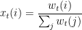
For this, it is convenient to return to the notation that we used in describing the multiplicative weights algorithm, that is, it is convenient to work with the weights defined as

$\displaystyle w_1(i) = 1$

$\displaystyle w_{t+1} (i) = w_t (i) \cdot e^{ \ell_t (i) / c}$

so that, at each time step

$\displaystyle x_t(i) = \frac {w_t(i)}{\sum_j w_t (j) }$

We are assuming ${0 \leq \ell_t (i) \leq 1}$ , so the weights are non-increasing with time. Then

$\displaystyle x_{t+1} (i) = \frac {w_{t+1} (i) }{\sum_j w_{t+1} (j) } = \frac {w_{t} (i) e^{-\ell_t (i) /c }}{\sum_j w_{t+1} (j) } \geq \frac {w_{t} (i) e^{-\ell_t (i) /c }}{\sum_j w_{t} (j) } \geq x_t(i) \cdot e^{-1/c}$

For every ${c \geq 1}$ we have ${e^{-1/c} \geq 1 - 1/c}$ , so

$\displaystyle x_{t}(i) - x_{t+1}(i) \leq \frac 1c x_t (i)$

and

$\displaystyle \langle \ell_t , x_t - x_{t+1} \rangle \leq \sum_i \ell_t(i) \cdot \frac 1c x_t(i) \leq \frac 1c$

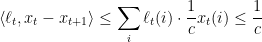
Putting it all together, we have

$\displaystyle {\rm Regret}_T \leq \frac Tc + c \ln n$

Choosing ${c = \sqrt{\frac T {\ln n}}}$ , we have

$\displaystyle {\rm Regret}_T \leq 2 \sqrt{T \ln n}$

Thus, we have reconstructed the analysis of the multiplicative weights algorithm.

Interestingly, the analysis that we derived today is not exactly identical to the one from the post on multiplicative weights. There, we derived the bound

$\displaystyle {\rm Regret}_T \leq \epsilon \sum_{t=1}^T \sum_{i=1}^n \ell_t^2 (i) x_t (i) \ + \frac {\ln n}{\epsilon }$

while here, setting ${\epsilon = 1/c}$ , we derived

$\displaystyle {\rm Regret}_T \leq \epsilon \sum_{t=1}^T \sum_{i=1}^n \ell_t (i) x_t(i) + \frac {\ln n}{\epsilon } - \frac 1 \epsilon H(x^*)$

where ${x^*}$ is the offline optimum and ${H(x) = \sum_i x_i \ln \frac 1 {x_i}}$ is the entropy function (computed using natural logarithms).

3. L2 Regularization

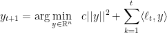
Now that we have a general method, let us apply it to a new context: suppose that, as before, our cost functions are linear, but let ${K = {\mathbb R}^n}$ . With linear cost functions and no bound on the size of solutions, it will not be possible to talk about regret with respect to the offline optimum, because the offline optimum will always be ${-\infty}$ , but it will be possible to talk about regret with respect to a particular offline solution ${x}$ , which will already lead to interesting consequences.

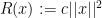
What regularizer should we use? In reasoning about regularizers, it can be helpful to think about what would go wrong if we use FTL, and then considering what regularizer would successfully “pull away” from the bad solutions found by FTL. In this context of linear loss functions and unbounded solutions, FTL will pick an infinitely big solution at each step, or, to be more precise, the “max” in the definition of FTL is undefined. To fight this tendency of FTL to go off to infinity, it makes sense for the regularizer to be a measure of how big a solution is. Since we are going to have to compute derivatives, it is good to use a measure of “bigness” with a nice gradient, and ${||x ||^2}$ is a natural choice. So, for a scale parameter ${c}$ to be optimized later, our regularizer will be

$\displaystyle R(x) := c || x||^2$

This tells us that

$\displaystyle x_ 1 = {\bf 0}$

and

$\displaystyle x_{t+1} = \arg\min_{x \in {\mathbb R}^n} \ \ c ||x||^2 + \sum_{k=1}^t \langle \ell_k , x \rangle$

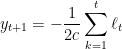
The function that we are minimizing in the above expression is convex, so we just have to compute the gradient and set it to zero

$\displaystyle 2c x + \sum_{k=1}^t \ell_k = 0$

$\displaystyle x = - \frac 1 {2c} \sum_{k=1}^t \ell_k$

Which can be also expressed as

$\displaystyle x_1 = {\bf 0}; \ \ \ x_{t+1} = x_t - \frac 1 {2c} \ell_t$

This makes perfect sense because, in the “experts” interpretation, we want to penalize the experts that performed badly in the past. Here we have no constraints on our allocations, so we simply decrease (additively this time, not multiplicatively) the allocation to the experts that caused a higher loss.

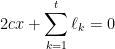
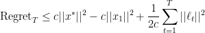
To compute the regret bound, we have

$\displaystyle f_t(x_t) - f_{t} (x_{t+1}) = \langle \ell_t, x_t - x_{t+1} \rangle = \left\langle \ell_t , \frac 1 {2c} \ell_t \right\rangle = \frac 1 {2c} || \ell_t||^2 ||$

and so the regret with respect to a solution ${x}$ is

$\displaystyle {\rm Regret}_T(x) \leq R(x) - R(x_1) + \sum_{t=1}^T f_t(x_t) - f_{t} (x_{t+1} )$

$\displaystyle = c || x||^2 + \frac 1 {2c} \sum_{t=1}^T || \ell_t||^2$

If we know a bound

$\displaystyle \forall t: \ \ || \ell_t || \leq L$

$\displaystyle || x|| \leq D$

then we can optimize ${c = \sqrt{\frac T {2D^2 L^2}}}$ and we have

$\displaystyle {\rm Regret}_T(x) \leq D L \sqrt{ 2 T}$

3.1. Dealing with Constraints

Consider now the case in which the loss functions are linear and ${K}$ is an arbitrary convex set. Using the same regularizer ${R(x) = c || x||^2}$ we have the algorithm

$\displaystyle x_1 = \arg\min_{x\in K} c ||x ||^2$

$\displaystyle x_{t+1} = \arg\min_{x\in K} \ \ c ||x ||^2 + \sum_{k=1}^{t} \langle \ell_t , x \rangle$

How can we solve the above constrained optimization problem? A very helpful observation is that we can first solve the unconstrained optimization and then project on ${K}$ , that is we can proceed as follows:

$\displaystyle y_{t+1} = \arg\min_{y\in {\mathbb R}^n} \ \ c ||y ||^2 + \sum_{k=1}^{t} \langle \ell_t , y \rangle$

$\displaystyle x'_{t+1} = \Pi_K (y_{t+1} ) = \arg\min_{x\in K} || x - y_{t+1} ||$

and we claim that we always have ${x'_{t+1} = x_{t+1}}$ . The fact that we can reduce a regularized constrained optimization problem to an unconstrained problem and a projection is part of a broader theory that we will describe in a later post. For now, we will limit to prove the equivalence in this specific setting. First of all, we already have an expression for ${y_{t+1}}$ , namely

$\displaystyle y_{t+1} = - \frac 1{2c} \sum_{k=1}^t \ell_t$

Now the definition of ${x'_{t+1}}$ is

$\displaystyle x'_{t+1} = \arg\min_{x\in K} || x - y_{t+1} ||$

$\displaystyle = \arg\min_{x\in K} || x - y_{t+1} ||^2$

$\displaystyle = \arg\min_{x\in K} ||x||^2 - 2 \left \langle x , y_{t+1} \right\rangle + || y_{t+1} ||^2$

$\displaystyle = \arg\min_{x\in K} ||x||^2 - 2 \left \langle x , y_{t+1} \right\rangle$

$\displaystyle = \arg\min_{x\in K} ||x||^2 - 2 \left\langle x , \frac 1{2c} \sum_{k=1}^t \ell_t \right\rangle$

$\displaystyle = \arg\min_{x\in K} c ||x||^2 - \sum_{k=1}^t \left\langle x , \ell_t \right\rangle = x_{t+1}$

In order to bound the regret, we have to compute

$\displaystyle f_t(x_t) - f_t(x_{t+1} ) = \langle \ell_t , x_t - x_{t+1} \rangle \leq || \ell_t || \cdot ||x_t - x_{t+1} ||$

and since L2 projections cannot increase L2 distances, we have

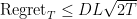
$\displaystyle || x_t - x_{t+1} || \leq || y_t - y_{t+1} || = \frac 1 {2c} || \ell_t ||$

So the regret bound is

$\displaystyle {\rm Regret}_T \leq c ||x^*||^2 - c|| x_1||^2 + \frac 1 {2c} \sum_{t=1}^T || \ell_t ||^2$

If ${D}$ is an upper bound to ${\max_{x\in K} || x||}$ , and ${L}$ is an upper bound to the norm ${|| \ell_t ||}$ of all the loss vectors, then

$\displaystyle {\rm Regret}_T \leq c D^2 + \frac 1 {2c} T L^2$

which can be optimized to

$\displaystyle {\rm Regret}_T \leq DL \sqrt {2T}$

3.2. Deriving the Analysis of Gradient Descent

Suppose that ${g: K \rightarrow {\mathbb R}}$ is a convex function whose gradient ${\nabla g}$ is well defined at all points in ${K}$ , and that we are interested in minimizing ${g}$ . Then a way to reduce this problem to online optimization would be to use the function ${g}$ as loss function at each step. Then the offline optimum would be the minimizer of ${g}$ , and achieving small regret means that ${\frac 1T \sum_t g(x_t)}$ is close to the minimum of ${g}$ , and so the best ${x_t}$ is an approximate minimizer.

Unfortunately, this is not a very helpful idea, because if we ran an FTRL algorithm against an adversary that keeps proposing ${g}$ as a cost function at each step then we would have

$\displaystyle x_{t+1} = \arg\min_{x\in K} R(x) + t \cdot g(x)$

which, for large ${t}$ , is essentially the same problem as minimizing ${g}$ , so we have basically reduced the problem of minimizing ${g}$ to itself.

Indeed, the power of the FTRL algorithm is that the algorithm does well even though it does not know the cost function, and if we keep using the same cost function at each step we are not making a good use of its power. Now, suppose that we use cost functions ${f_t}$ such that

${f_t(x_t) = g(x_t)}$
${\forall x\in K \ \ f_t(x) \leq g(x)}$

Then, after ${T}$ steps, we have

$\displaystyle \sum_{t=1}^T g(x_t) = \sum_{t=1}^T f_t(x_t) = {\rm Regret}_T + \min{x\in K} \sum_{t=1}^T f_t(x) \leq {\rm Regret}_T + \min_{x\in K} \sum_{t=1}^T g (x)$

meaning

$\displaystyle \frac 1T \sum_{t=1}^T g(x_t) \leq \frac {{\rm Regret}_T}T + \min_{x\in K} g(x)$

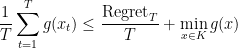
and so one of the ${x_t}$ is an approximate minimizer. Indeed, using convexity, we also have

$\displaystyle g \left( \frac 1T \sum_{t=1}^T x_t \right) \leq \frac 1T \sum_{t=1}^T g(x_t) \leq \frac {{\rm Regret}_T}T + \min_{x\in K} g(x)$

and so the average of the ${x_t}$ is also an approximate minimizer. From the point of view of exploiting FTRL do to minimize ${g}$ , cost functions ${f_t}$ as above work just as well as presenting ${g}$ as a cost functions at each step.

How do we find cost functions that satisfy the above two properties and for which the FTRL algorithm is easy to implement? The idea is to let ${f_t}$ be the linear approximation of ${g}$ at ${x_t}$ :

$\displaystyle f_t (x) := g(x_t) + \langle \nabla g (x_t), x - x_t \rangle$

The ${f_t(x_t) = g(x_t)}$ condition is immediate, and

$\displaystyle g(x) \geq f_t (x)$

is a consequence of the convexity of ${g}$ .

The cost functions that we have defined are affine functions, that is, each of them equals a constant plus a linear function

$\displaystyle f_t(x) = \left( g(x_t) - \langle \nabla g(x_t) , x_t\rangle \right) + \langle \nabla g(x_t) , x \rangle$

Adding a constant term to a cost function does not change the iteration of FTRL, and does not change the regret (because the same term is added both to the solution found by the algorithm and to the offline optimum), so the algorithm is just initialized with

$\displaystyle y_1 = {\bf 0}$

$\displaystyle x_1 = \Pi_K({\bf 0}) = \arg\min_{x\in K} || x||$

and then continues with the update rules

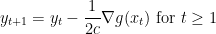
$\displaystyle y_{t+1} =y_t -\frac 1 {2c} \nabla g (x_t) \mbox{ for } t \geq 1$

$\displaystyle x_{t+1} = \Pi_K(y_{t+1}) = \arg\min_{x\in K} || x - y_{t+1} || \mbox{ for } t \geq 1$

which is just projected gradient descent.

If we have known upper bounds

$\displaystyle \forall x \in K \ \ || \nabla g(x) || \leq L$

and

$\displaystyle \forall x \in K \ \ || x || \leq D$

then we have

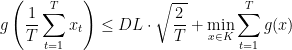
$\displaystyle g \left( \frac 1 T \sum_{t=1}^T x_t \right ) \leq DL \cdot \sqrt{\frac 2 T} + \min_{x\in K} \sum_{t=1}^T g (x)$

which means that to achieve additive error ${\epsilon}$ it is enough to proceed for ${2D^2L^2 / \epsilon^2}$ steps.

3 thoughts on “Online Optimization Post 3: Follow the Regularized Leader”

Nicolò Campolongo on August 1, 2019 at 5:09 am said:

Hi Luca, I think there’s a typo in “Negative Entropy Regularization” section. When you say:

“With this choice of regularizer, we have: $$ x_t = \argmin_{x \in Delta} \sum_{k=1}^{t-1} \langle \ell_k, x_k \rangle + … $$ ”

But the $k$ subscript shouldn’t be there for the x in the inner product, right? And also later, same thing: “the constraint {x \in \Delta} reduces to {\sum_i x_i = 1}, so we have to consider the function

$$ \left( \sum_{k=1}^{t-1} \langle \ell_k , x_k \rangle \right ) + … $$ “
anon on September 21, 2019 at 8:28 am said:

Thanks for the posts, very educational and cool. You write great motivated math.
Pingback: Online Optimization Post 7: Matrix Multiplicative Weights Update | in theory

in theory

"Marge, I agree with you – in theory. In theory, communism works. In theory." — Homer Simpson

Online Optimization Post 3: Follow the Regularized Leader

3 thoughts on “Online Optimization Post 3: Follow the Regularized Leader”

Leave a comment

Share this:

Related

3 thoughts on “Online Optimization Post 3: Follow the Regularized Leader”

Leave a comment