In which we show how to use linear programming to approximate the vertex cover problem.
1. Linear Programming Relaxations
An integer linear program (abbreviated ILP) is a linear program (abbreviated LP) with the additional constraints that the variables must take integer values. For example, the following is an ILP:

Where 
If we are interested in designing a polynomial time algorithm (exact or approximate) for a combinatorial optimization problem, formulating the combinatorial optimization problem as an ILP is useful as a first step in the following methodology (the discussion assumes that we are working with a minimization problem):
- Formulate the combinatorial optimization problem as an ILP;
- Derive a LP from the ILP by removing the constraint that the variables have to take integer value. The resulting LP is called a “relaxation” of the original problem. Note that in the LP we are minimizing the same objective function over a larger set of solutions, so
;
- Solve the LP optimally using an efficient algorithm for linear programming;
- If the optimal LP solution has integer values, then it is a solution for the ILP of cost
, and so we have found an optimal solution for the ILP and hence an optimal solution for our combinatorial optimization problem;
- If the optimal LP solution
has fractional values, but we have a rounding procedure that transforms
such that
for some constant
, then we are able to find a solution to the ILP of cost
, and so we have a
- If the optimal LP solution has integer values, then it is a solution for the ILP of cost
In this lecture and in the next one we will see how to round fractional solutions of relaxations of the Vertex Cover and the Set Cover problem, and so we will be able to derive new approximation algorithms for Vertex Cover and Set Cover based on linear programming.
2. The Weighted Vertex Cover Problem
Recall that in the vertex cover problem we are given an undirected graph 


We described the following 2-approximate algorithm:
- Input:
-
- For each
- if
then
- if
- return


The algorithm finds a vertex cover by construction, and if the condition in the if step is satisfied 


Our simple algorithm can perform very badly on weighted instances. For example consider the following graph:

Then the algorithm would start from the edge 


Why does the approximation analysis fail in the weighted case? In the unweighted case, every edge which is considered by the algorithm must cost at least 1 to the optimum solution to cover (because those edges form a matching), and our algorithm invests a cost of 2 to cover that edge, so we get a factor of 2 approximation. In the weighted case, an edge in which one endpoint has cost 1 and one endpoint has cost 100 tells us that the optimum solution must spend at least 1 to cover that edge, but if we want to have both endpoints in the vertex cover we are going to spend 101 and, in general, we cannot hope for any bounded approximation guarantee.
We might think of a heuristic in which we modify our algorithm so that, when it considers an uncovered edge in which one endpoint is much more expensive than the other, we only put the cheaper endpoint in
Indeed, it is rather tricky to approximate the weighted vertex cover problem via a combinatorial algorithm, although we will develop (helped by linear programming intuition) such an approximation algorithm by the end of the lecture.
Developing a 2-approximate algorithm for weighted vertex cover via a linear programming relaxation, however, is amazingly simple.
3. A Linear Programming Relaxation of Vertex Cover
Let us apply the methodology described in the first section. Given a graph 


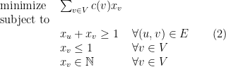
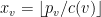
Next, we relax the ILP (2) to a linear program.

Let us solve the linear program in polynomial time, and suppose that 


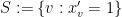
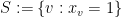
- The set
, and so at least one of
or
must be at least
, and so at least one of
- The cost of


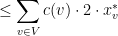


And that’s all there is to it! We now have a polynomial-time 2-approximate algorithm for weighted vertex cover.
4. The Dual of the LP Relaxation
The vertex cover approximation algorithm based on linear programming is very elegant and simple, but it requires the solution of a linear program. Our previous vertex cover approximation algorithm, instead, had a very fast linear-time implementation. Can we get a fast linear-time algorithm that works in the weighted case and achieves a factor of 2 approximation? We will see how to do it, and although the algorithm will be completely combinatorial, its analysis will use the LP relaxation of vertex cover.
How should we get started in thinking about a combinatorial approximation algorithm for weighted vertex cover?
We have made the following point a few times already, but it is good to stress it again: in order to have any hope to design a provably good approximation algorithm for a minimization problem, we need to have a good technique to prove lower bounds for the optimum. Otherwise, we will not be able to prove that the optimum is at least a constant fraction of the cost of the solution found by our algorithms.
In the unweighted vertex cover problem, we say that if a graph has a matching of size
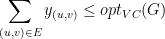
How else can we prove lower bounds? Well, how did we establish a lower bound to the optimum in our LP-based 2-approximate algorithm? We used the fact that the optimum of the linear programming relaxation (3) is a lower bound to the minimum vertex cover optimum. The next idea is to observe that the cost of any feasible solution to the dual of (3) is a lower bound to the optimum of (3), by weak duality, and hence a lower bound to the vertex cover optimum as well.
Let us construct the dual of (3). Before starting, we note that if we remove the 

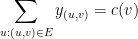
Its dual has one variable 

That is, we want to assign a nonnegative “charge”
Example 1 (Matchings) Suppose that we have an unweighted graph
is a matching. Then we can define
if
and
if
. This is a feasible solution for (5) of cost
.
This means that any lower bound to the optimum in the unweighted case via matchings can also be reformulated as lower bounds via feasible solutions to (5). The latter approach, however, is much more powerful.
Example 2 Consider the weighted star graph from Section 2. We can define
for each vertex
, and this is a feasible solution to (5). This proves that the vertex cover optimum is at least 5.
5. Linear-Time 2-Approximation of Weighted Vertex Cover
Our algorithm will construct, in parallel, a valid vertex cover 

- Input: undirected, unweighted, graph
-
-
- for each edge
- if
and
then
-
- if
-
- return


Our goal is to modify the above algorithm so that it can deal with vertex weights, while maintaining the property that it finds an integral feasible 


We will get simpler formulas if we think in terms of a new set of variables 


Initially, we start from the all-zero dual solution 


Here is the psedocode of the algorithm:
- Input: undirected, unweighted, graph
-
-
- for each edge
- if
-
- if
-
- return


The algorithm outputs a correct vertex cover, because for each edge 
Clearly, we have

Next, we claim that the vector

because initially all the

by construction, and so the charges
and define a feasible dual solution. We then have
by weak duality. Finally, every time we give a value to a

Putting all together we have
and we have another 2-approximate algorithm for weighted vertex cover!
It was much more complicated than the simple rounding scheme applied to the linear programming optimum, but it was worth it because now we have a linear-time algorithm, and we have understood the problem quite a bit better.
