CS261 Lecture 18: Using Expert Advice

In which we show how to use expert advice, and introduce the powerful “multiplicative weight” algorithm.

We study the following online problem. We have ${n}$ “experts” that, at each time step ${t=1,\ldots,T}$ , suggest a strategy about what to do at that time (for example, they might be advising on what technology to use, on what investments to make, they might make predictions on whether something is going to happen, thus requiring certain actions, and so on). Based on the quality of the advice that the experts offered in the past, we decide which advice to follow, or with what fraction of our investment to follow which strategy. Subsequently, we find out which loss or gain was associated to each strategy, and, in particular, what loss or gain we personally incurred with the strategy or mix of strategies that we picked, and we move to step ${t+1}$ .

We want to come up with an algorithm to use the expert advice such that, at the end, that is, at time ${T}$ , we are about as well off as if we had known in advance which expert was the one that gave the best advice, and we had always followed the strategy suggested by that expert at each step. Note that we make no probabilistic assumption, and our analysis will be a worst-case analysis over all possible sequences of events.

The “multiplicative update” algorithm provides a very good solution to this problem, and the analysis of this algorithm is a model for the several other applications of this algorithm, in rather different contexts.

1. A Simplified Setting

We begin with the following simplified setting: at each time step, we have to make a prediction about an event that has two possible outcomes, and we can use the advice of ${n}$ “experts,” which make predictions about the outcome at each step. Without knowing anything about the reliability of the experts, and without making any probabilistic assumption on the outcomes, we want to come up with a strategy that will lead us to make not much more mistakes than the “offline optimal” strategy of picking the expert which makes the fewest mistakes, and then always following the prediction of that optimal expert.

The algorithm works as follows: at each step ${t}$ , it assigns a weight ${w_i^t}$ to each expert ${i}$ , which measures the confidence that the algorithm has in the validity of the prediction of the expert. Initially, ${w^0_i = 1}$ for all experts ${i}$ . Then the algorithm makes the prediction that is backed by the set of experts with largest total weight. For example, if the experts, and us, are trying to predict whether the following day it will rain or not, we will look at the sum of the weights of the experts that say it will rain, and the sum of the weights of the experts that say it will not, and then we agree with whichever prediction has the largest sum of weights. After the outcome is revealed, we divide by 2 the weight of the experts that were wrong, and leave the weight of the experts that were correct unchanged.

We now formalize the above algorithm in pseudocode. We use ${\{a,b\}}$ to denote the two possible outcomes of the event that we are required to predict at each step.

for each ${i\in \{1,\ldots, n\}}$ do ${w^1_i:= 1}$
for each time
- let ${w^t := \sum_i w_i^t}$
- if the sum of ${w^t_i}$ over all the experts ${i}$ that predict ${a}$ is ${\geq w^t/2}$ , then predict ${a}$
- else predict ${b}$
- wait until the outcome is revealed
- for each
  - if ${i}$ was wrong then ${w^{t+1}_i := w^{t}_i/2}$

To analyze the algorithm, let ${m_i^t}$ be the indicator variable that expert ${i}$ was wrong at time ${t}$ , that is, ${m_i^t=1}$ if the expert ${i}$ was wrong at time ${i}$ and ${m_i^t=0}$ otherwise. (Here ${m}$ stands for “mistake.”) Let ${m_i = \sum_{t=1}^T m_i^t}$ be the total number of mistakes made by expert ${i}$ . Let ${m_A^t}$ be the indicator variable that our algorithm makes a mistake at time ${t}$ , and ${m_A:= \sum_{t=1}^T m_A^t}$ be the total number of mistakes made by our algorithm.

We make the following two observations:

If the algorithm makes a mistake at time ${t}$ , then the total weight of the experts that are mistaken at time ${t}$ is ${\geq w^{t}/2}$ , and, at the following step, the weight of those experts is divided by two, and this means that, if we make a mistake at time ${t}$ then
$\displaystyle w^{t+1} \leq \frac 34 w^{t}$

Because the initial total weight is ${w^1 = n}$ , we have that, at the end,

$\displaystyle w^{T+1} \leq \left( \frac 34 \right) ^{m_A} \cdot n$
For each expert ${i}$ , the final weight is ${w^{T+1}_i = 2^{-m_i}}$ , and, clearly,
$\displaystyle \frac 1 {2^{m_i}} = w_i^{T+1} \leq w^{T+1}$

Together, the two previous observations mean that, for every expert ${i}$ ,

$\displaystyle \frac 1 {2^{m_i}} \leq \left( \frac 34 \right) ^{m_A} \cdot n$

which means that, for every expert ${i}$ ,

$\displaystyle m_A \leq O(m_i + \log n)$

That is, the number of mistakes made by the algorithm is at most a constant times the number of mistakes of the best expert, plus an extra ${O(\log n)}$ mistakes.

We will now discuss an algorithm that improves the above result in two ways. We will show that, for every ${\epsilon}$ , the improved algorithm we can make the number of mistakes be at most ${(1+\epsilon) m_i + O\left( \frac 1 \epsilon \log n \right)}$ for every ${\epsilon}$ , which can be seen to be optimal for small ${n}$ , and the improved algorithm will be able to handle a more general problem, in which the experts are suggesting arbitrary strategies, and the outcome of each strategy can be an arbitrary gain or loss.

2. The General Result

We now consider the following model. At each time step ${t}$ , each expert ${i}$ suggests a certain strategy. We choose to follow the advice of expert ${i}$ with probability ${p^t_i}$ , or, equivalently, we allocate a ${p^t_i}$ fraction of our resources in the way expert ${i}$ advised. Then we observe the outcome of the strategies suggested by the experts, and of our own strategy. We call ${m_i^t}$ the loss incurred by following the advice of expert ${i}$ . The loss can be negative, in which case it is a gain, and we normalize losses and gains so that ${m_i^t \in [-1,1]}$ for every ${i}$ and every ${t}$ . Our own loss for the time step ${t}$ will then be ${\sum_i p_i^t m_i^t}$ . At the end, we would like to say that our own sum of losses is not much higher than the sum of losses of the best expert.

As before, our algorithm maintains a weight for each expert, corresponding to our confidence in the expert. The weights are initialized to 1. When an expert causes a loss, we reduce his weight, and when an expert causes a gain, we increase his weight. To express the weight updated in a single instruction, we have 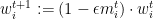${w^{t+1}_i := (1-\epsilon m_i^t) \cdot w^t_i}$ , where ${0 < \epsilon < 1/2}$ is a parameter of our choice. Our probabilities ${p^t_i}$ are chosen proportionally to weights ${w^t_i}$ .

for each ${i\in \{1,\ldots, n\}}$ do ${w^1_i:= 1}$
for each time
- let ${w^t := \sum_i w_i^t}$
- let ${p^t_i := w_i^t/ w^t}$
- for each ${i}$ , follow the strategy of expert ${i}$ with probability ${p^t_i}$
- wait until the outcome is revealed
- let ${m^t_i}$ be the loss of the strategy of expert ${i}$
- for each
  - ${w^{t+1}_i := (1 - \epsilon \cdot m_i^t ) \cdot w^t_i}$

To analyze the algorithm, we will need the following technical result.

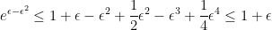
Fact 1 For every ${\epsilon \in [-1/2,1/2]}$ ,

$\displaystyle e^{\epsilon - \epsilon^2} \leq 1+\epsilon \leq e^{\epsilon}$

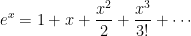
Proof: We will use the Taylor expansion

$\displaystyle e^{x} = 1 + x + \frac {x^2}2 + \frac{x^3}{3!} + \cdots$

The upper bound. The Taylor expansion above can be seen as ${e^x = 1 + x + \sum_{t=1}^\infty x^{2t} \cdot \left( \frac {1}{(2t)!} + \frac{x}{(2t+1)!} \right)}$ , that is, ${e^x}$ equals ${1+x}$ plus a sum of terms that are all non-negative when ${x\geq -1}$ . Thus, in particular, we have ${1+\epsilon \leq e^{\epsilon}}$ for ${\epsilon \in [-1/2,1/2]}$ .
The lower bound for positive ${\epsilon}$ . We can also see that, for ${x\in [0,1]}$ , we have
$\displaystyle e^x \leq 1 + x + x^2$

and so, for ${\epsilon \in [0,1]}$ we have

$\displaystyle e^{\epsilon-\epsilon^2} \leq 1 + \epsilon - \epsilon^2 + \epsilon^2 - 2\epsilon^3 + \epsilon^4 \leq 1 + \epsilon$
The lower bound for negative ${\epsilon}$ . Finally, for ${x\in [-1,0]}$ we have
$\displaystyle e^x = 1 + x + \frac {x^2}2 + \sum_{t=1}^\infty x^{2t + 1} \left( \frac 1{(2t+1)!} + \frac x {(2t+2)!} \right) \leq 1 + x + \frac {x^2} 2$

and so, for ${\epsilon \in [-1/2,0]}$ we have

$\displaystyle e^{\epsilon - \epsilon^2} \leq 1 + \epsilon - \epsilon^2 + \frac 12 \epsilon^2 - \epsilon^3 + \frac 14 \epsilon^4 \leq 1 + \epsilon$

$\Box$

Now the analysis proceeds very similarly to the analysis in the previous section. We let

$\displaystyle m_A^t := \sum_i p_i^t m_i^t$

be the loss of the algorithm at time ${t}$ , and ${m_A := \sum_{t=1}^T m_A^t}$ the total loss at the end. We denote by ${m_i:= \sum_{t=1}^T m_i^t}$ the total loss of expert ${i}$ .

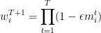
If we look at the total weight at time ${t+1}$ , it is

$\displaystyle w^{t+1} = \sum_i w^{t+1}_i = \sum_i (1- \epsilon m_i^t) \cdot w^t_i$

and we can rewrite it as

$\displaystyle w^{t+1} = w^t - \sum_i \epsilon m_i^t w^t_i = w^t - w^t \epsilon \cdot \sum_i m_i^t p_i^t = w^t \cdot ( 1- \epsilon m_A^t)$

Recalling that, initially, ${w^1 = n}$ , we have that the total weight at the end is

$\displaystyle w^{T+1} = n \cdot \prod_{t=1}^T (1 - \epsilon m_A^t)$

For each expert ${i}$ , the weight of that expert at the end is

$\displaystyle w^{T+1}_i = \prod_{t=1}^T (1-\epsilon m_i^t)$

and, as before, we note that for every expert ${i}$ we have

$\displaystyle w^{T+1}_i \leq w^{T+1}$

Putting everything together, for every expert ${i}$ we have

$\displaystyle \prod_{t=1}^T (1-\epsilon m_i^t) \leq n \cdot \prod_{t=1}^T (1 - \epsilon m_A^t)$

Now it is just a matter of taking logarithms and of using the inequality that we proved before.

$\displaystyle \ln \prod_{t=1}^T (1 - \epsilon m_A^t) = \sum_{i=1}^T \ln 1 - \epsilon m_A^t \leq - \sum_{i=1}^T \epsilon m_A^t = - \epsilon m_A$

$\displaystyle \ln \prod_{t=1}^T (1-\epsilon m_i^t) = \sum_{t=1}^T \ln 1-\epsilon m_i^T \geq \sum_{t=1}^T - \epsilon m_i^t - \epsilon^2 (m_i^t)^2$

and, overall,

$\displaystyle m_A \leq + m_i + \epsilon \sum_{i=1}^T |m_i^t| +\frac{\ln n}{\epsilon} \ \ \ \ \ (1)$

In the model of the previous section, at every step the loss of each expert is either 0 or 1, and so the above expression simplifies to

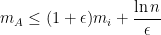
$\displaystyle m_A \leq (1+ \epsilon) m_i + \frac {\ln n } {\epsilon}$

which shows that we can get arbitrarily close to the best expert.

In every case, (1) simplifies to

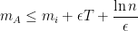
$\displaystyle m_A \leq m_i + \epsilon T + \frac {\ln n }{\epsilon}$

and, if we choose ${\epsilon = \sqrt{\ln n/T}}$ , we have

$\displaystyle m_A \leq m_i + 2 \sqrt{T\ln n}$

which means that we come close to the optimum up to a small additive error.

To see that this is essentially the best that we can hope for, consider a playing a fair roulette game as follows: for ${T}$ times, we either bet $1 on red or $1 on black. If we win we win $1, and if we lose we lose $1; we win and lose with probability 1/2 each at each step. Clearly, for every betting strategy, our expected win at the end is 0. We can think of the problem as there being two experts: the red expert always advises to bet red, and the black expert always advises to bet black. For each run of the game, the strategy of always following the best expert has a non-negative gain and, on average, following the best expert has a gain of ${\Omega( \sqrt{T})}$ , because there is ${\Omega(1)}$ probability that the best expert has a gain of ${\Omega(\sqrt T)}$ . This means that we cannot hope to always achieve at least the gain of the best expert minus ${o(\sqrt T)}$ , even in a setting with 2 experts.

3. Applications

The general expert setting is very similar to a model of investments in which the experts correspond to stocks (or other investment vehicles) and the outcomes correspond to the variation in value of the stocks. The difference is that in our model we “invest” one unit of money at each step regardless of what happened in previous steps, while in investment strategies we compound our gains (and losses). If we look at the logarithm of the value of our investment, however, it is modeled correctly by the experts setting.

The multiplicative update algorithm that we described in the previous section arises in several other contexts, with a similar, or even identical, analysis. For example, it arises in the context of boosting in machine learning, and it leads to efficient approximate algorithms for certain special cases of linear programming.

2 thoughts on “CS261 Lecture 18: Using Expert Advice”

Xamuel on March 18, 2011 at 7:44 pm said:

Very interesting article. As a logician I’m particularly interested in the case when T=infinity. In particular, I’m interested in the case when the “experts” are really expert trolls and are intentionally trying to confuse us. For example, say that, in addition to trying to determine whether it will rain tomorrow, we also have a “secondary mission” which is to determine which expert is the most reliable. For simplicity, assume there are only two experts, A and B, both who have perfect knowledge of the weather. Rather than perfectly predict it, though, they conspire together so that A makes correct predictions and B makes incorrect ones until we eventually suspect A is the best expert. Then, they switch, A making incorrect predictions and B making correct predictions, until we suspect that B is the best expert. This continues indefinitely, forcing us to change our minds infinitely often. And contrary to intuition, it does NOT require the experts be able to see our guesses, provided we’ve nailed down the multiplicative weight algorithm or any other particular algorithm. The experts can merely run that algorithm themselves, allowing them to confuse us even if our guesses are invisible to them. It would be interesting to compute exactly what predictions these mischievous experts would make (this is completely determined, assuming, say, that by coincidence it rains every day).
xyz on March 19, 2011 at 7:34 pm said:

Some corrections:

1. In both the simplified and general settings, it seems w_{i}^{1} should be 1, not 0.

2. The inequality signs (\leq, \geq) just above the statement of Eq. (1) should be reversed.

[Thanks, fixed now. — L.]

in theory

"Marge, I agree with you – in theory. In theory, communism works. In theory." — Homer Simpson

CS261 Lecture 18: Using Expert Advice

2 thoughts on “CS261 Lecture 18: Using Expert Advice”

Leave a comment

Share this:

Related

2 thoughts on “CS261 Lecture 18: Using Expert Advice”

Leave a comment