CS359G Lecture 3: Cheeger’s inequality

In which we prove the easy case of Cheeger’s inequality.

1. Expansion and The Second Eigenvalue

Let ${G=(V,E)}$ be an undirected ${d}$ -regular graph, ${A}$ its adjacency matrix, ${M = \frac 1d \cdot A}$ its normalized adjacency matrix, and ${1=\lambda_1 \geq \lambda_2 \geq \cdots \geq \lambda_n}$ be the eigenvalues of ${M}$ .

Recall that we defined the edge expansion of a cut ${(S,V-S)}$ of the vertices of ${G}$ as

$\displaystyle h(S) := \frac {E(S,V-S)}{d \cdot \min \{ |S|, |V-S| \} }$

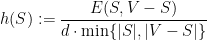
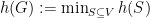
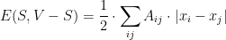
and that the edge expansion of ${G}$ is ${h(G) := \min_{S\subseteq V} h(S)}$ .

We also defined the related notion of the sparsity of a cut ${(S,V-S)}$ as

$\displaystyle \phi(S) := \frac {E(S,V-S)}{ \frac dn \cdot |S| \cdot |V-S| }$

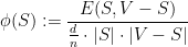
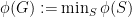
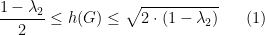
and ${\phi(G) := \min_S \phi(S)}$ ; the sparsest cut problem is to find a cut of minimal sparsity.

Recall also that in the last lecture we proved that ${\lambda_2 = 1}$ if and only if ${G}$ is disconnected. This is equivalent to saying that ${1-\lambda_2 = 0 }$ if and only if ${h(G)=0}$ . In this lecture and the next we will see that this statement admits an approximate version that, qualitatively, says that ${1-\lambda_2}$ is small if and only if ${h(G)}$ is small. Quantitatively, we have

Theorem 1 (Cheeger’s Inequalities)

$\displaystyle \frac{1-\lambda_2}2 \leq h(G) \leq \sqrt{2 \cdot (1-\lambda_2) } \ \ \ \ \ (1)$

2. The Easy Direction

In this section we prove

Lemma 2 ${1-\lambda_2 \leq \phi(G)}$

From which we have one direction of Cheeger’s inequality, after recalling that ${\phi(G) \leq 2 h(G)}$ .

Let us find an equivalent restatement of the sparsest cut problem. If represent a set ${S\subseteq V}$ as a bit-vector ${x\in \{ 0,1 \}^V}$ , then

$\displaystyle E(S,V-S) = \frac 12 \cdot \sum_{ij} A_{ij} \cdot |x_i - x_j|$

and

$\displaystyle |S| \cdot |V-S| = \frac 12 \cdot \sum_{ij} |x_i - x_j|$

so that, after some simplifications, we can write

$\displaystyle \phi(G) = \min_{{\bf x} \in \{ 0,1 \}^V -\{ {\bf {0}},{\bf 1} \} } \frac { \sum_{ij} M_{ij} | x_i - x_j | } { \frac 1n \sum_{ij} |x_i - x_j | } \ \ \ \ \ (2)$

Note that, when ${x_i,x_j}$ take boolean values, then so does ${|x_i - x_j|}$ , so that we may also equivalently write

$\displaystyle \phi(G) = \min_{{\bf x} \in \{ 0,1 \}^V -\{ {\bf {0}},{\bf 1} \} } \frac { \sum_{ij} M_{ij} | x_i - x_j |^2 } { \frac 1n \sum_{ij} |x_i - x_j | ^2} \ \ \ \ \ (3)$

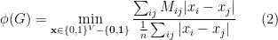
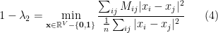
In the last lecture, we gave the following characterization of ${1-\lambda_2}$ :

$\displaystyle 1-\lambda_2 = \min_{{\bf x} \in {\mathbb R}^V-\{ {\bf {0}} \}, {\bf x} \perp {\bf 1}} \frac { \sum_{ij} M_{ij} | x_i - x_j |^2 } { 2 \cdot \sum_i x_i^2}$

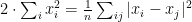
Now we claim that the following characterization is also true

$\displaystyle 1-\lambda_2 = \min_{{\bf x} \in {\mathbb R}^V-\{ {\bf {0}},{\bf 1} \} } \frac { \sum_{ij} M_{ij} | x_i - x_j |^2 } { \frac 1n \sum_{ij} |x_i - x_j | ^2} \ \ \ \ \ (4)$

This is because

$\displaystyle \sum_{i,j} |x_i - x_j|^2$

$\displaystyle = \sum_{ij} x_i^2 + \sum_{ij} x_j^2 - 2 \sum_{ij} x_ix_j$

$\displaystyle = 2n \sum_i x_i^2 - 2 \left( \sum_i x_i \right)^2$

so for every ${{\bf x} \in {\mathbb R}^V - \{ {\bf {0}}\}}$ such that ${{\bf x} \perp {\bf 1}}$ we have that ${2 \cdot \sum_i x_i^2 = \frac 1n \sum_{ij} |x_i-x_j|^2}$ , and so

$\displaystyle \min_{{\bf x} \in {\mathbb R}^V-\{ {\bf {0}} \}, {\bf x} \perp {\bf 1}} \frac { \sum_{ij} M_{ij} | x_i - x_j |^2 } { 2 \cdot \sum_i x_i^2} = \min_{{\bf x} \in {\mathbb R}^V-\{ {\bf {0}} \} , {\bf x} \perp {\bf 1}} \frac { \sum_{ij} M_{ij} | x_i - x_j |^2 } { \frac 1n \sum_{ij} |x_i - x_j | ^2} \$

To conclude the argument, take an ${{\bf x}}$ that maximized the right-hand side of (4), and observe that if we shift every coordinate by the same constant then we obtain another optimal solution, because the shift will cancel in all the expressions both in the numerator and the denominator. In particular, we can define ${{\bf x}'}$ such that ${x'_i = x_ i - \frac 1n \sum_j x_j}$ and note that the entries of ${{\bf x}'}$ sum to zero, and so ${{\bf x}' \perp {\bf 1}}$ . This proves that

$\displaystyle \min_{{\bf x} \in {\mathbb R}^V-\{ {\bf {0}} \} , {\bf x} \perp {\bf 1}} \frac { \sum_{ij} M_{ij} | x_i - x_j |^2 } { \frac 1n \sum_{ij} |x_i - x_j | ^2} = \min_{{\bf x} \in {\mathbb R}^V-\{ {\bf {0}},{\bf 1} \} } \frac { \sum_{ij} M_{ij} | x_i - x_j |^2 } { \frac 1n \sum_{ij} |x_i - x_j | ^2}$

and so we have established (4).

Comparing (4) and (3), it is clear that the quantity ${1-\lambda_2}$ is a continuous relaxation of ${\phi(G)}$ , and hence ${1-\lambda_2 \leq \phi(G)}$ .

3. Other Relaxations of ${\phi(G)}$

Having established that we can view ${1-\lambda_2}$ as a relaxation of ${\phi(G)}$ , the proof that ${h(G) \leq \sqrt{2 \cdot (1-\lambda_2)}}$ can be seen as a rounding algorithm, that given a real-valued solution to (4) finds a comparably good solution for (3).

Later in the course we will see two more approximation algorithms for sparsest cut and edge expansion. Both are based on continuous relaxations of ${\phi}$ starting from (2).

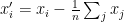
The algorithm of Leighton and Rao is based on a relaxation that is defined by observing that every bit-vector ${{\bf x} \in \{ 0,1 \}^V}$ defines the semi-metric ${d(i,j) := |x_i - x_j|}$ over the vertices; the Leighton-Rao relaxation is obtained by allowing arbitrary semi-metrics:

$\displaystyle LR(G) := \min_{\begin{array}{l} d: V \times V \rightarrow {\mathbb R}\\ d \ {\rm semimetric} \end{array}} \frac { \sum_{ij} M_{ij} d(i,j) } {\frac 1n \sum_{ij} d(i,j) }$

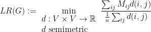
It is not difficult to express ${LR(G)}$ as a linear programming problem.

The algorithm of Arora-Rao-Vazirani is obtained by noting that, for a bit-vector ${x\in \{ 0,1 \}^V}$ , the distances ${d(i,j) := |x_i - x_j|}$ define a metric which can also be seen as the Euclidean distance between the ${x_i}$ , because ${|x_i - x_j| = \sqrt{(x_i - x_j)^2}}$ , and such that ${d^2(i,j)}$ is also a semi-metric, trivially so because ${d^2(i,j) = d(i,j)}$ . If a distance function ${d(\cdot,\cdot)}$ is a semi-metric such that ${\sqrt{d(\cdot,\cdot)}}$ is a Euclidean semi-metric, then ${d(\cdot,\cdot)}$ is called a negative type semi-metric. The Arora-Rao-Vazirani relaxation is

$\displaystyle ARV(G) := \min_{\begin{array}{l} d: V \times V \rightarrow {\mathbb R}\\ d \ {\rm negative\ type\ semimetric} \end{array}} \frac { \sum_{ij} M_{ij} d(i,j) } {\frac 1n \sum_{ij} d(i,j) }$

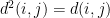
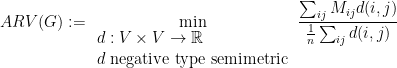
The Arora-Rao-Vazirani relaxation can be expressed as a semi-definite programming problem.

From this discussion it is clear that the Arora-Rao-Vazirani relaxation is a tightening of the Leigthon-Rao relaxation and that we have

$\displaystyle \phi(G) \geq ARV(G) \geq LR(G)$

It is less obvious in this treatment, and we will see it later, that the Arora-Rao-Vazirani is also a tightening of the relaxation of ${\phi}$ given by ${1-\lambda_2}$ , that is

$\displaystyle \phi(G) \geq ARV(G) \geq 1 - \lambda_2$

The relaxations ${1-\lambda_2}$ and ${LR(G)}$ are incomparable.

4 thoughts on “CS359G Lecture 3: Cheeger’s inequality”

Anon on January 23, 2011 at 8:09 pm said:

Do you know if there is a version of Cheeger’s inequality that relates to non-uniform sparsest cut?
Pingback: Lecture 8 « Pseudorandomness and Derandomization
Pingback: Lecture 9 « Pseudorandomness and Derandomization
Pingback: Superexpanders: part 1 | Probability, Geometry & Group Theory blog

Enter your comment here...

Fill in your details below or click an icon to log in:

Email (required) (Address never made public)

Name (required)

Website

You are commenting using your WordPress.com account. ( Log Out / Change )

You are commenting using your Twitter account. ( Log Out / Change )

You are commenting using your Facebook account. ( Log Out / Change )

Cancel

Connecting to %s

in theory

"Marge, I agree with you – in theory. In theory, communism works. In theory." — Homer Simpson

CS359G Lecture 3: Cheeger’s inequality

4 thoughts on “CS359G Lecture 3: Cheeger’s inequality”

Leave a Reply

Share this:

Like this:

Related

4 thoughts on “CS359G Lecture 3: Cheeger’s inequality”

Leave a Reply