CS261 Lecture 15: the LP of Max Flow

In which we look at the linear programming formulation of the maximum flow problem, construct its dual, and find a randomized-rounding proof of the max flow – min cut theorem.

In the first part of the course, we designed approximation algorithms “by hand,” following our combinatorial intuition about the problems. Then we looked at linear programming relaxations of the problems we worked on, and we saw that approximation algorithms for those problems could also be derived by rounding a linear programming solution. We also saw that our algorithms could be interpreted as constructing, at the same time, an integral primal solution and a feasible solution for the dual problem.

Now that we have developed exact combinatorial algorithms for a few problems (maximum flow, minimum s-t cut, global min cut, maximum matching and minimum vertex cover in bipartite graphs), we are going to look at linear programming relaxations of those problems, and use them to gain a deeper understanding of the problems and of our algorithms.

We start with the maximum flow and the minimum cut problems.

1. The LP of Maximum Flow and Its Dual

Given a network ${(G=(V,E), s, t, c)}$ , the problem of finding the maximum flow in the network can be formulated as a linear program by simply writing down the definition of feasible flow.

We have one variable ${f(u,v)}$ for every edge ${(u,v)\in E}$ of the network, and the problem is:

$\displaystyle \begin{array}{lll} \mbox{maximize} & \displaystyle\sum_{v: (s,v)\in E} f(s,v)\\ \mbox{subject to}\\ &\displaystyle \sum_{u: (u,v)\in E} f(u,v) = \sum_{w: (v,w)\in E} f(v,w) & \forall v \in V- \{s,t\}\\ & f(u,v) \leq c(u,v) & \forall (u,v) \in E\\ & f(u,v) \geq 0 & \forall (u,v) \in E \end{array} \ \ \ \ \ (1)$

Now we want to construct the dual.

When constructing the dual of a linear program, it is often useful to rewrite it in a way that has a simpler structure, especially if it is possible to rewrite it in a way that has fewer constraints (which will correspond to fewer dual variables), even at the cost of introducing several new variables in the primal.

A very clean way of formulating the maximum flow problem is to think in terms of the paths along which we are going to send the flow, rather than in terms of how much flow is passing through a specific edge, and this point of view makes the conservation constraints unnecessary.

In the following formulation, we have one variable ${x_p}$ for each of the possible simple paths from ${s}$ to ${t}$ (we denote by ${P}$ the set of such paths), specifying how much of the flow from ${s}$ to ${t}$ is being routed along the path ${p}$ :

$\displaystyle \begin{array}{lll} \mbox{maximize} & \displaystyle\sum_{p \in P} x_p\\ \mbox{subject to}\\ & \displaystyle \sum_{p\in P : (u,v) \in p} x_p \leq c(u,v) & \forall (u,v) \in E\\ & x_p \geq 0 & \forall p \in P \end{array} \ \ \ \ \ (2)$

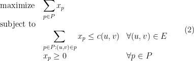
Note that, usually, a network has exponentially many possible paths from ${s}$ to ${t}$ , and so the linear program (2) has an exponential number of variables. This is ok because we are never going to write down (2) for a specific network and pass it to a linear programming solver; we are interested in (2) as a mathematical specification of the maximum flow problem. If we want to actually find a maximum flow via linear programming, we will use the equivalent formulation (1).

(There are several other cases in combinatorial optimization in which a problem has a easier-to-understand linear programming relaxation or formulation that is exponentially big, and one can prove that it is equivalent to another relaxation or formulation of polynomial size. One then proves theorems about the big linear program, and the theorems apply to the small linear program as well, because of the equivalence. Then the small linear program can be efficiently solved, and the theorems about the big linear program can be turned into efficient algorithms.)

Let us first confirm that indeed (1) and (2) are equivalent.

Fact 1 If ${f(\cdot,\cdot)}$ is a feasible solution for (1), then there is a feasible solution for (2) of the same cost.

Proof: Note that this is exactly the Flow Decomposition Theorem that we proved in Lecture 11, in which it is stated as Lemma 2. $\Box$

Fact 2 If ${\{ x_p \}_{p\in P}}$ is a feasible solution for (2), then there is a feasible solution for (1) of the same cost.

Proof: Define

$\displaystyle f(u,v) := \sum_{p\in P: (u,v) \in p} x_p$

that is, let ${f(u,v)}$ the sum of the flows of all the paths that use the edge ${(u,v)}$ . Then ${f(\cdot,\cdot)}$ satisfies the capacity constraints and, regarding the conservation constraints, we have

$\displaystyle \sum_{u: (u,v) \in E} f(u,v) = \sum_{p\in P: v\in p} x_p = \sum_{w: (v,w)\in E} f(u,v)$

$\Box$

Let us now construct the dual of (2). We have one dual variable ${y_{u,v}}$ for every edge ${(u,v) \in E}$ , and the linear program is:

$\displaystyle \begin{array}{lll} \mbox{minimize} & \displaystyle\sum_{(u,v) \in E} c(u,v) y_{u,v}\\ \mbox{subject to}\\ & \displaystyle \sum_{(u,v) \in p} y_{u,v} \geq 1 & \forall p\in P\\ & y_{u,v} \geq 0 & \forall (u,v)\in E \end{array} \ \ \ \ \ (3)$

The linear program (3) is assigning a weight to each edges, which we may think of as a “length,” and the constraints are specifying that, along each possible path, ${s}$ and ${t}$ are at distance at least one. This means that dual variables are expressing a way of “separating” ${s}$ from ${t}$ and, after thinking about it for a moment, we see that (3) can be seen as a linear programming relaxation of the minimum cut problem.

Fact 3 For every feasible cut ${A}$ in the network ${(G,s,t,c)}$ , there is a feasible solution ${\{ y_{u,v} \}_{(u,v)\in E}}$ to (3) whose cost is the same as the capacity of ${A}$ .

Proof: Define ${y_{u,v}=1}$ if ${u\in A}$ and ${v\not\in A}$ , and let ${y_{u,v}=0}$ otherwise. Then

$\displaystyle \sum_{u,v} c(u,v) y_{u,v} = \sum_{u\in A, v\not\in A} c(u,v) = capacity(A)$

$\Box$

This means that the optimum of (3) is smaller than or equal to the capacity of the minimum cut in the network. Now we are going to describe a randomized rounding method that shows that the optimum of (3) is actually equal to the capacity of the minimum cut. Since the optimum of (3) is equal to the optimum of (2) by the Strong Duality Theorem, and we have proved that the optimum of (3) is equal to the cost of the maximum flow of the network, Lemma 4 below will prove that the cost of the maximum flow in the network is equal to the capacity of the minimum flow, that is, it will be a different proof of the max flow – min cut theorem. It is actually a more difficult proof (because it uses the Strong Duality Theorem whose proof, which we have skipped, is not easy), but it is a genuinely different one, and a useful one to understand, because it gives an example of how to use randomized rounding to solve a problem optimally. (So far, we have only seen examples of the use of randomized rounding to design approximate algorithms.)

Lemma 4 Given any feasible solution ${\{ y_{u,v} \}_{(u,v) \in E}}$ to (3), it is possible to find a cut ${A}$ such that

$\displaystyle capacity(A) \leq \sum_{u,v} c(u,v) y_{u,v}$

Proof: Interpret the ${y_{u,v}}$ as weights on the edges, and use Dijkstra’s algorithm to find, for every vertex ${v}$ , the distance ${d(v)}$ from ${s}$ to ${v}$ according to the weights ${y_{u,v}}$ .

The constraints in (3) imply that ${d(t) \geq 1}$ .

Pick a value ${T}$ uniformly at random in the interval ${[0,1)}$ , and let ${A}$ be the set

$\displaystyle A:= \{ v : d(v) \leq T \}$

Then, for every choice of ${T}$ , ${A}$ contains ${s}$ and does not contain ${t}$ , and so it is a feasible cut.

Using linearity of expectation, the average (over the choice of ${T}$ ) capacity of ${A}$ can be written as

$\displaystyle \mathop{\mathbb E}_{T \sim [0,1)} capacity(A) = \sum_{(u,v)\in E} c(u,v) \mathop{\mathbb P} [ u\in A \wedge v\not\in A]$

and

$\displaystyle \mathop{\mathbb P} [ u\in A \wedge v\not\in A ] = \mathop{\mathbb P} [ d(u) \leq T < d(v) ] = d(v)-d(u)$

Finally, we observe the “triangle inequality”

$\displaystyle d(v) \leq d(u) + y_{u,v}$

which says that the shortest path from ${s}$ to ${v}$ is at most the length of the shortest path from ${s}$ to ${u}$ plus the length of the edge ${(u,v)}$ .

Putting all together, we have

$\displaystyle \mathop{\mathbb E}_{T \sim [0,1)} capacity(A) \leq \sum_{(u,v)\in E} c(u,v) y_{u,v}$

and there clearly must exist a choice of ${T}$ for which the capacity of ${A}$ is at most the expected capacity.

About finding ${A}$ efficiently, we can also note that, although there is an infinite number of choices for ${T}$ , there are only at most ${|V|-1}$ different cuts that can be generated. If we sort the vertices in increasing order of ${d(v)}$ , and let them be ${u_1,\ldots,u_{|V|}}$ in this order, then we have ${s=u_1}$ , and let ${k}$ be such that ${d(u_k)< 1}$ but ${d(u_{k+1}) \geq 1}$ . Then the only cuts which are generated in our probability distribution are the ${k}$ cuts of the form

$\displaystyle A_i := \{ s=u_1,u_2,\ldots,u_i \}$

for ${i=1,\ldots, k}$ , and one of them must have capacity ${\leq \sum_{(u,v) \in E} y_{u,v}c(u,v)}$ . We can compute the capacity of each ${A_i}$ and pick the ${A_i}$ with the smallest capacity. $\Box$

Let us now see what the dual of (1) looks like. It will look somewhat more mysterious than (3), but now we know what to expect: because of the equivalence between (1) and (2), the dual of (1) will have to be a linear programming relaxation of the minimum cut problem, and it will have an exact randomized rounding procedure.

The dual of (1) has one variable for each vertex ${v}$ (except ${s}$ and ${t}$ ), which we shall call ${y_v}$ , corresponding to the conservation constraints, and one variable for each edge, which we shall call ${y_{u,v}}$ , corresponding to the capacity constraints.

$\displaystyle \begin{array}{lll} \mbox{minimize} & \displaystyle\sum_{(u,v) \in E} c(u,v) y_{u,v}\\ \mbox{subject to}\\ & y_v + y_{s,v} \geq 1 & \forall v : (s,v) \in E\\ & y_v - y_u + y_{u,v} \geq 0 & \forall (u,v)\in E, u\neq s, v\neq t\\ & - y_u + y_{u,t} \geq 0 & \forall u : (u,t) \in E \end{array} \ \ \ \ \ (4)$

Let us see that (4) is a linear programming relaxation of the minimum cut problem and that it admits an exact rounding algorithm.

Fact 5 If ${A}$ is a feasible cut in the network, then there is a feasible solution to (4) such that

$\displaystyle capacity(A) = \sum_{(u,v) \in E} c(u,v) y_{u,v}$

Proof: Define ${y_{v} = 1}$ if ${v\in A}$ , and ${y_v = 0}$ if ${v\not\in A}$ . Define ${y_{u,v} = 1}$ if ${u\in A}$ and ${v\not \in A}$ , and ${y_{u,v} = 0}$ otherwise.

To see that it is a feasible solution, let us first consider the constraints of the first kind. They are always satisfied because if ${v\in A}$ then ${y_v=1}$ , and if ${v\not \in A}$ then ${(s,v)}$ crosses the cut and ${y_{s,v} =1}$ , so the left-hand-side is always at least one. We can similarly see that the constraints of the third type are satisfied.

Regarding the constraints of the second kind, we can do a case analysis and see that the constraint is valid if ${y_u=0}$ (regardless of the value of the other variables), and it is also valid if ${y_v=1}$ (regardless of the value of the other variables). The remaining case is ${y_u=1}$ and ${y_v=0}$ , which is the case in which ${(u,v)}$ crosses the cut and so ${y_{u,v} =1}$ . $\Box$

Fact 6 Given a feasible solution of (4), we can find a feasible cut whose capacity is equal to the cost of the solution.

Proof: Pick uniformly at random ${T}$ in ${[0,1]}$ , then define

$\displaystyle A:= \{ s \} \cup \{ v: y_v \geq T \}$

This is always a cut, because, by construction, it contains ${s}$ and it does not contain ${t}$ . (Recall that there is no variable ${y_t}$ because there is no conservation constraint for ${t}$ .)

Then we have

$\displaystyle \mathop{\mathbb E} capacity(A) = \sum_{u,v} c(u,v) \mathop{\mathbb P} [ u\in A \wedge v \not \in A ]$

It remains to argue that, for every edge ${(u,v)}$ , we have

$\displaystyle \mathop{\mathbb P} [ u\in A \wedge v \not \in A ] \leq y_{u,v}$

For edges of the form ${(s,v)}$ , we have

$\displaystyle \mathop{\mathbb P} [ s\in A \wedge v \not \in A ] = \mathop{\mathbb P} [ v \not\in A ] = \mathop{\mathbb P} [ y_v < T \leq 1 ] = 1-y_v \leq y_{s,v}$

(Actually, the above formula applies if ${0\leq y_v < 1}$ . If ${y_v \geq 1}$ , then the probability is zero and ${y_{s,v} \geq 0}$ and we are fine; if ${y_v < 0}$ , then the probability is one, and ${y_{s,v} \geq 1-y_v > 1}$ , so we are again fine.)

For edges of the form ${(u,v)}$ in which ${u}$ and ${v}$ are in ${V-\{ s,t\}}$ we have

$\displaystyle \mathop{\mathbb P} [ u \in A \wedge v \not \in A] = \mathop{\mathbb P} [ y_v < T \leq y_u ] = y_u-y_v \leq y_{u,v}$

(Again, we have to look out for various exceptional cases, such as the case ${y_v\geq y_u}$ , in which case the probability is zero and ${y_{u,v} \geq 0}$ , and the case ${y_v < 0}$ , and the case ${y_u>1}$ .)

For edges of the form ${(v,t)}$ , we have

$\displaystyle \mathop{\mathbb P} [ v\in A \wedge t \not \in A ] = \mathop{\mathbb P} [ v \in A ] = \mathop{\mathbb P} [ y_v \geq T ] = y_v \leq y_{v,t}$

(Same disclaimers.) $\Box$

1 thought on “CS261 Lecture 15: the LP of Max Flow”

aram on November 22, 2011 at 9:43 pm said:

If you’re working with an optimal solution of the LP in (3) then you don’t even need to optimize over all cuts; any threshold in (0,1) will work deterministically.

in theory

"Marge, I agree with you – in theory. In theory, communism works. In theory." — Homer Simpson

CS261 Lecture 15: the LP of Max Flow

1 thought on “CS261 Lecture 15: the LP of Max Flow”

Leave a Reply Cancel reply

Share this:

Like this:

Related

1 thought on “CS261 Lecture 15: the LP of Max Flow”

Leave a Reply Cancel reply