Scribed by Luowen Qian
In which we use spectral techniques to find certificates of unsatisfiability for random  -SAT formulas.
1. Introduction
Given a random -SAT formula with  clauses and
  variables, we want to find a certificate of unsatisfiability of such formula within polynomial time. Here we consider as fixed, usually equal to 3 or 4. For fixed , the more clauses you have, the more constraints you have, so it becomes easier to show that these constraints are inconsistent. For example, for 3-SAT,
- In the previous lecture, we have shown that if
 for some large constant
  , almost surely the formula is not satisfiable. But it’s conjectured that there is no polynomial time, or even subexponential time algorithms that can find the certificate of unsatisfiability for
  .
.
- If
 for some other constant
  , we’ve shown in the last time that we can find a certificate within polynomial time with high probability that the formula is not satisfiable.
The algorithm for finding such certificate is shown below.
- Algorithm 3SAT-refute(
 )
)
- for

- if 2SAT-satisfiable( restricted to clauses that contains
 , with
  )
)
- return

- return UNSATISFIABLE
We know that we can solve 2-SATs in linear time, and approximately

clauses contains  . Similarly when is sufficiently large, the 2-SATs will almost surely be unsatisfiable. When a subset of the clauses is not satisfiable, the whole 3-SAT formula is not satisfiable. Therefore we can certify unsatisfiability for 3-SATs with high probability.
In general for -SAT,
- If
 for some large constant
  , almost surely the formula is not satisfiable.
- If
 for some other constant
  , we can construct a very similar algorithm, in which we check all assignments to the first
  variables, and see if the 2SAT part of the restricted formula is unsatisfiable.
Since for every fixed assignments to the first  variables, approximately

portion of the clauses remains, we expect the constant  and the running time is
  .
.
So what about ‘s that are in between? It turns out that we can do better with spectral techniques. And the reason that spectral techniques work better is that unlike the previous method, it does not try all the possible assignments and fails to find a certificate of unsatisfiability.
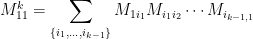
2. Reduce certifying unsatisfiability for k-SAT to finding largest independent set
2.1. From 3-SAT instances to hypergraphs
Given a random 3-SAT formula , which is an and of random 3-CNF-SAT clauses over variables  (abbreviated as vector
  ), i.e.

where ![{\sigma_{i,j} \in [n], b_{i,j} \in \{0, 1\}}](https://s0.wp.com/latex.php?latex=%7B%5Csigma_%7Bi%2Cj%7D+%5Cin+%5Bn%5D%2C+b_%7Bi%2Cj%7D+%5Cin+%5C%7B0%2C+1%5C%7D%7D&bg=ffffff&fg=000000&s=0&c=20201002) ,
, ![{\forall i \in [m], \sigma_{i,1} < \sigma_{i,2} < \sigma_{i,3}}](https://s0.wp.com/latex.php?latex=%7B%5Cforall+i+%5Cin+%5Bm%5D%2C+%5Csigma_%7Bi%2C1%7D+%3C+%5Csigma_%7Bi%2C2%7D+%3C+%5Csigma_%7Bi%2C3%7D%7D&bg=ffffff&fg=000000&s=0&c=20201002) and no two
and no two  are exactly the same. Construct hypergraph
  , where
![\displaystyle X = \left\{(i, b) \middle| i \in [n], b \in \{0, 1\}\right\}](https://s0.wp.com/latex.php?latex=%5Cdisplaystyle+X+%3D+%5Cleft%5C%7B%28i%2C+b%29+%5Cmiddle%7C+i+%5Cin+%5Bn%5D%2C+b+%5Cin+%5C%7B0%2C+1%5C%7D%5Cright%5C%7D&bg=ffffff&fg=000000&s=0&c=20201002)
is a set of  vertices, where each vertex means an assignment to a variable, and
![\displaystyle E = \left\{ e_j \middle| j \in [m] \right\}, e_j = \{(\sigma_{j,1}, \overline{b_{j,1}}), (\sigma_{j,2}, \overline{b_{j,2}}), (\sigma_{j,3}, \overline{b_{j,3}})\}](https://s0.wp.com/latex.php?latex=%5Cdisplaystyle+E+%3D+%5Cleft%5C%7B+e_j+%5Cmiddle%7C+j+%5Cin+%5Bm%5D+%5Cright%5C%7D%2C+e_j+%3D+%5C%7B%28%5Csigma_%7Bj%2C1%7D%2C+%5Coverline%7Bb_%7Bj%2C1%7D%7D%29%2C+%28%5Csigma_%7Bj%2C2%7D%2C+%5Coverline%7Bb_%7Bj%2C2%7D%7D%29%2C+%28%5Csigma_%7Bj%2C3%7D%2C+%5Coverline%7Bb_%7Bj%2C3%7D%7D%29%5C%7D&bg=ffffff&fg=000000&s=0&c=20201002)
is a set of 3-hyperedges. The reason we’re putting in the negation of  is that a 3-CNF clause evaluates to false if and only if all three subclauses evaluate to false. This will be useful shortly after.
First let’s generalize the notion of independent set for hypergraphs.
An independent set for hypergraph  is a set
  that satisfies
  .
.
If is satisfiable,  has an independent set of size at least . Equivalently if the largest independent set of has size less than , is unsatisfiable. Proof: Assume is satisfiable, let
  be a satisfiable assignment, where
  . Then
 ![{S = \{ (x_i, y_i) | i \in [n] \}}](https://s0.wp.com/latex.php?latex=%7BS+%3D+%5C%7B+%28x_i%2C+y_i%29+%7C+i+%5Cin+%5Bn%5D+%5C%7D%7D&bg=ffffff&fg=000000&s=0&c=20201002) is an independent set of size . If not, it means some hyperedge
is an independent set of size . If not, it means some hyperedge  , so
, so  and the
  -th clause in evaluates to false. Therefore evaluates to false, which contradicts the fact that
  is a satisfiable assignment.
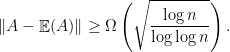
We know that if we pick a random graph that’s sufficiently dense, i.e. the average degree  , by spectral techniques we will have a certifiable upper bound on the size of the largest independent set of
  with high probability. So if a random graph has
  random edges, we can prove that there’s no large independent set with high probability.
But if we have a random hypergraph with random hyperedges, we don’t have any analog of spectral theories for hypergraphs that allow us to do this kind of certification. And from the fact that the problem of certifying unsatisfiability of random formula of clauses is considered to be hard, we conjecture that there doesn’t exist a spectral theory for hypergraphs able to replicate some of the things we are able to do on graphs.
However, what we can do is possibly with some loss, to reduce the hypergraph to a graph, where we can apply spectral techniques.
2.2. From 4-SAT instances to graphs
Now let’s look at random 4-SATs. Similarly we will write a random 4-SAT formula as:

where , ![{\forall i \in [m], \sigma_{i,1} < \sigma_{i,2} < \sigma_{i,3} < \sigma_{i,4}}](https://s0.wp.com/latex.php?latex=%7B%5Cforall+i+%5Cin+%5Bm%5D%2C+%5Csigma_%7Bi%2C1%7D+%3C+%5Csigma_%7Bi%2C2%7D+%3C+%5Csigma_%7Bi%2C3%7D+%3C+%5Csigma_%7Bi%2C4%7D%7D&bg=ffffff&fg=000000&s=0&c=20201002) and no two
and no two  are exactly the same. Similar to the previous construction, but instead of constructing another hypergraph, we will construct just a graph
  , where
![\displaystyle V = \left\{(i_1, b_1, i_2, b_2) \middle| i_1, i_2 \in [n], b_1, b_2 \in \{0, 1\}\right\}](https://s0.wp.com/latex.php?latex=%5Cdisplaystyle+V+%3D+%5Cleft%5C%7B%28i_1%2C+b_1%2C+i_2%2C+b_2%29+%5Cmiddle%7C+i_1%2C+i_2+%5Cin+%5Bn%5D%2C+b_1%2C+b_2+%5Cin+%5C%7B0%2C+1%5C%7D%5Cright%5C%7D&bg=ffffff&fg=000000&s=0&c=20201002)
is a set of  vertices and
![\displaystyle E = \left\{ e_j \middle| j \in [m] \right\}, e_j = \{(\sigma_{j,1}, \overline {b_{j,1}}, \sigma_{j,2}, \overline {b_{j,2}}), (\sigma_{j,3}, \overline {b_{j,3}}, \sigma_{j,4}, \overline {b_{j,4}})\}](https://s0.wp.com/latex.php?latex=%5Cdisplaystyle+E+%3D+%5Cleft%5C%7B+e_j+%5Cmiddle%7C+j+%5Cin+%5Bm%5D+%5Cright%5C%7D%2C+e_j+%3D+%5C%7B%28%5Csigma_%7Bj%2C1%7D%2C+%5Coverline+%7Bb_%7Bj%2C1%7D%7D%2C+%5Csigma_%7Bj%2C2%7D%2C+%5Coverline+%7Bb_%7Bj%2C2%7D%7D%29%2C+%28%5Csigma_%7Bj%2C3%7D%2C+%5Coverline+%7Bb_%7Bj%2C3%7D%7D%2C+%5Csigma_%7Bj%2C4%7D%2C+%5Coverline+%7Bb_%7Bj%2C4%7D%7D%29%5C%7D&bg=ffffff&fg=000000&s=0&c=20201002)
is a set of edges.
If is satisfiable,  has an independent set of size at least
  . Equivalently if the largest independent set of has size less than , is unsatisfiable. Proof: The proof is very similar to the previous one. Assume is satisfiable, let be a satisfiable assignment, where . Then
 ![{S = \{ (x_i, y_i, x_j, y_j) | i, j \in [n] \}}](https://s0.wp.com/latex.php?latex=%7BS+%3D+%5C%7B+%28x_i%2C+y_i%2C+x_j%2C+y_j%29+%7C+i%2C+j+%5Cin+%5Bn%5D+%5C%7D%7D&bg=ffffff&fg=000000&s=0&c=20201002) is an independent set of size . If not, it means some edge , so
is an independent set of size . If not, it means some edge , so  and the -th clause in evaluates to false. Therefore evaluates to false, which contradicts the fact that is a satisfiable assignment.
From here, we can observe that is not a random graph because some edges are forbidden, for example when the two vertices of the edge has some element in common. But it’s very close to a random graph. In fact, we can apply the same spectral techniques to get a certifiable upper bound on the size of the largest independent set if the average degree , i.e. if  , we can certify unsatisfiability with high probability, by upper bounding the size of the largest independent set in the constructed graph.
We can generalize this results for all even ‘s. For random -SAT where is even, if  , we can certify unsatisfiability with high probability, which is better than the previous method which requires
  . The same
  is achievable for odd , but the argument is significantly more complicated.
2.3. Certifiable upper bound for independent sets in modified random sparse graphs
Despite odd ‘s, another question is that in this setup, can we do better and get rid of the  term? This term is coming from the fact that spectral norm break down when the average degree
  . However it’s still true that random graph doesn’t have any large independent sets even when the average degree
  is constant. It’s just that the spectral norm isn’t giving us good bounds any more, since the spectral norm is at most
  . So is there something tighter than spectral bounds that could help us get rid of the term? Could we fix this by removing all the high degree vertices in the random graph?
This construction is due to Feige-Ofek. Given random graph  , where the average degree
  is some large constant. Construct
  by taking
  and removing all edges incident on nodes with degree higher than
  where
where  is the average degree of . We denote
  for the adjacency matrix of and
  for that of . And it turns out,
With high probability,  .
.
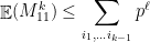
It turns out to be rather difficult to prove. Previously we saw spectral results on random graphs that uses matrix traces to bound the largest eigenvalue. In this case, it’s hard to do so because the contribution to the trace of a closed walk is complicated by the fact that edges have dependencies. The other approach is that given random matrix  , we will try to upper bound
  . A standard way for this is to that for every solution, count the instances of in which the fixed solution is good, and argue that the number of the fixed solutions is small, which tells us that there’s no good solution. The problem here is that the set of solutions is infinitely large. So Feige-Ofek discretize the set of vectors, and then reduce the bound on the quadratic form of a discretized vector to a sum of several terms, each of which has to be carefully bounded.
We always have

and so, with high probability, we get an  polynomial time upper bound certificate to the size of the independent set for a
  random graph. This removes the extra term from our analysis of certificates of unsatisfiability for random -SAT when is even.
3. SDP relaxation of independent sets in random sparse graphs
In order to show a random graph has no large independent sets, a more principled way is to argue that there is some polynomial time solvable relaxation of the problem whose solution is an upper bound of the problem.
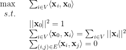
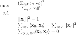
Let SDPIndSet be the optimum of the following semidefinite programming relaxation of the Independent Set problem, which is due to Lovász:

Since it’s the relaxation of the problem of finding the maximum independent set,  for any graph . And this relaxation has a nice property.
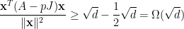
For every  , and for every graph , we have \begin{equation*} {\rm SDPIndSet}(G) \leq \frac 1p \cdot || pJ – A || \end{equation*} where
  is the all-one matrix and is the adjacency matrix of .
Proof: First we note that SDPIndSet is at most
and this is equal to
which is at most

because

Finally, the above optimization is equivalent to the following

which is at most the unconstrained problem

Recall from the previous section that we constructed by removing edges from , which corresponds to removing constraints in our semidefinite programming problem, so  , which is by theorem 3 at most with high probability.
4. SDP relaxation of random k-SAT
From the previous section, we get an idea that we can use semidefinite programming to relax the problem directly and find a certificate of unsatisfiability for the relaxed problem.
Given a random -SAT formula :

The satisfiability of is equivalent of the satisfiability of the following equations:
![\displaystyle \begin{array}{rcl} && x_i^2 = x_i \forall i \in [n] \\ && \sum_{i = 1}^m \left(1 - \prod_{j = 1}^k\left((-1)^{b_{i,j}}x_{\sigma_{i,j}} + b_{i,j}\right)\right) = m \end{array}](https://s0.wp.com/latex.php?latex=%5Cdisplaystyle++%5Cbegin%7Barray%7D%7Brcl%7D++%26%26+x_i%5E2+%3D+x_i+%5Cforall+i+%5Cin+%5Bn%5D+%5C%5C+%26%26+%5Csum_%7Bi+%3D+1%7D%5Em+%5Cleft%281+-+%5Cprod_%7Bj+%3D+1%7D%5Ek%5Cleft%28%28-1%29%5E%7Bb_%7Bi%2Cj%7D%7Dx_%7B%5Csigma_%7Bi%2Cj%7D%7D+%2B+b_%7Bi%2Cj%7D%5Cright%29%5Cright%29+%3D+m+%5Cend%7Barray%7D+&bg=ffffff&fg=000000&s=0&c=20201002)
Notice that if we expand the polynomial on the left side, there are some of the monomials having degree higher than 2 which prevents us relaxing these equations to a semidefinite programming problem. In order to resolve this,  and
and  we introduce
  . Then we can relax all variables to be vectors, i.e.
For example, if we have a 4-SAT clause

we can rewrite it as

For this relaxation, we have:
- If
 , the SDP associated with the formula is feasible with high probability, where
  for every fixed .
- If
 , the SDP associated with the formula is not feasible with high probability, where
  is a constant for every fixed even , and
  for every fixed odd .
 with an unknown partition of the vertices into two equal parts
  and
and  . Edges across the partition are generated independently with probability
  , and edges inside the partition are generated independently with probability
  . To abbreviate the notation, we let
  , which is the average internal degree, and
  , which is the average external degree. Intuitively, the closer are
  and
and  , although there are also similar results in the complementary model where
  so that the graph is not almost empty.
 , there exists a constant
  such that if
 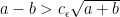 , then we can reconstruct the partition up to less than
  misclassified vertices.
  , then we can do exact reconstruct.
 such that if
  , then it will be impossible to reconstruct the partition even if an
  fraction of misclassified vertices is allowed. Also, the constant
  needs to be a bigger and bigger constant times
  . When the constant becomes
  , we will get an exact reconstruction as stated in the second result.
 problem
  is partitioned into two 2 subsets of equal size:
  . Then for
  pair of vertices in the same subset,
  and otherwise
  .
.  . If we want to find the partition
  has expected size
  and any other cut will have greater expected size.
 , the problem only gets harder. And for fixed ratio
  , as
, as  , the problem only gets easier. This can be stated rigorously as follows: If we can solve the problem for
  then we can also solve it for
  where
where  , by keeping only
  edges and reducing to the case we can solve.
 . We then defined
  as the vertices
  with the
  and cleaned up
  . Note this is intuitive as the average degree of the graph is
  . The idea is simple: Solve
 . At the end of this class, we wrapped up this topic and started the topic of
  with
with  . The following code describes a sampler for the distribution.


 , make
  if
if 
 otherwise
 , which is the case in which the planted clique is, with high probability, larger than any pre-existing clique
 are mutually independent random variables with values
  . \newline Let
  . The Chernoff Bounds claim the following: \newline
![\displaystyle \mathop{\mathbb P}(\vert X - \mathop{\mathbb E}[X] \vert) > \epsilon \cdot \mathop{\mathbb E}[X]) \leq \exp(\Omega(\epsilon^2 \cdot \mathop{\mathbb E}[X]))](https://s0.wp.com/latex.php?latex=%5Cdisplaystyle++%5Cmathop%7B%5Cmathbb+P%7D%28%5Cvert+X+-+%5Cmathop%7B%5Cmathbb+E%7D%5BX%5D+%5Cvert%29+%3E+%5Cepsilon+%5Ccdot+%5Cmathop%7B%5Cmathbb+E%7D%5BX%5D%29+%5Cleq+%5Cexp%28%5COmega%28%5Cepsilon%5E2+%5Ccdot+%5Cmathop%7B%5Cmathbb+E%7D%5BX%5D%29%29&bg=ffffff&fg=000000&s=0&c=20201002)

![\displaystyle \mathop{\mathbb P} (\vert X - \mathop{\mathbb E}[X] \vert \geq t \cdot \mathop{\mathbb E}[X]) \leq \exp(-\Omega((t\log(t)) \cdot \mathop{\mathbb E}[X]))](https://s0.wp.com/latex.php?latex=%5Cdisplaystyle++%5Cmathop%7B%5Cmathbb+P%7D+%28%5Cvert+X+-+%5Cmathop%7B%5Cmathbb+E%7D%5BX%5D+%5Cvert+%5Cgeq+t+%5Ccdot+%5Cmathop%7B%5Cmathbb+E%7D%5BX%5D%29+%5Cleq+%5Cexp%28-%5COmega%28%28t%5Clog%28t%29%29+%5Ccdot+%5Cmathop%7B%5Cmathbb+E%7D%5BX%5D%29%29&bg=ffffff&fg=000000&s=0&c=20201002)
![{\mathop{\mathbb E}[X]}](https://s0.wp.com/latex.php?latex=%7B%5Cmathop%7B%5Cmathbb+E%7D%5BX%5D%7D&bg=ffffff&fg=000000&s=0&c=20201002) , we can bound as follows:
, we can bound as follows: ![\displaystyle \mathop{\mathbb P}(\vert X - \mathop{\mathbb E}[X] \vert \geq \epsilon \cdot n) \leq \exp(- \Omega(\epsilon^2 \cdot n))](https://s0.wp.com/latex.php?latex=%5Cdisplaystyle++%5Cmathop%7B%5Cmathbb+P%7D%28%5Cvert+X+-+%5Cmathop%7B%5Cmathbb+E%7D%5BX%5D+%5Cvert+%5Cgeq+%5Cepsilon+%5Ccdot+n%29+%5Cleq+%5Cexp%28-+%5COmega%28%5Cepsilon%5E2+%5Ccdot+n%29%29+&bg=ffffff&fg=000000&s=0&c=20201002)
 Via SDP Rounding
  where
where  . We show that with
  probability, the max-degree will be
![\displaystyle \mathop{\mathbb P}(\textrm{v has degree} > c \cdot d) = \mathop{\mathbb P}(\vert deg(v) - \mathop{\mathbb E}[v] \vert > (c - 1) \mathop{\mathbb E}[deg(v)])](https://s0.wp.com/latex.php?latex=%5Cdisplaystyle+%5Cmathop%7B%5Cmathbb+P%7D%28%5Ctextrm%7Bv+has+degree%7D+%3E+c+%5Ccdot+d%29+%3D+%5Cmathop%7B%5Cmathbb+P%7D%28%5Cvert+deg%28v%29+-+%5Cmathop%7B%5Cmathbb+E%7D%5Bv%5D+%5Cvert+%3E+%28c+-+1%29+%5Cmathop%7B%5Cmathbb+E%7D%5Bdeg%28v%29%5D%29&bg=ffffff&fg=000000&s=0&c=20201002)


![\displaystyle \mathop{\mathbb E}[\textrm{number vertices in triangles}] = n \cdot \mathop{\mathbb P}(\textrm{v participates in a triangle})](https://s0.wp.com/latex.php?latex=%5Cdisplaystyle+%5Cmathop%7B%5Cmathbb+E%7D%5B%5Ctextrm%7Bnumber+vertices+in+triangles%7D%5D+%3D+n+%5Ccdot+%5Cmathop%7B%5Cmathbb+P%7D%28%5Ctextrm%7Bv+participates+in+a+triangle%7D%29&bg=ffffff&fg=000000&s=0&c=20201002)
 ways of choosing the other two vertices that participate with v in the triangle. \newline So the expected number of vertices in triangles can be bounded by
![\displaystyle \mathop{\mathbb E}[\textrm{number vertices in triangles}] \leq n \cdot p^3 \cdot \binom{n - 1}{2}](https://s0.wp.com/latex.php?latex=%5Cdisplaystyle++%5Cmathop%7B%5Cmathbb+E%7D%5B%5Ctextrm%7Bnumber+vertices+in+triangles%7D%5D+%5Cleq+n+%5Ccdot+p%5E3+%5Ccdot+%5Cbinom%7Bn+-+1%7D%7B2%7D&bg=ffffff&fg=000000&s=0&c=20201002)

 probability,
  vertices participate in triangles.
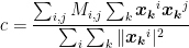
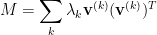
 be the largest eigenvalue of M:
  We can formulate this as Quadratic Programming:

 of SDP can hold as a solution to the QP and vice versa.
 . We note that our SDP can be transformed into an unconstrained optimization problem as follows:
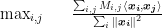

 element of


 . It’s obvious that
  . Under our constraints, we can rewrite our SDP as
 . Relaxing our constraint will yield an optimization problem with a solution less than the stricter constraint (call this
  ):
):
 . We can rewrite
 :
:
 ,
, 


 with high probability. This implies that
  . Semantically, this means that
  computes in poly-time a correct upper-bound of
  .
.  . The following are true:
  eigenvalues are
 ;
; 
 .
.

 is defined as the number of expected paths from
 . Since traces relates the sum of the diagonal and the sum of eigenvalues for symmetric
  , then with high probability
  , where
  is the spectral norm. Generally, if
  and
and  then w.h.p.
 ,
,
 signifies
  . Take
  such that
  .
. is defined to be
  where
where  matrix.
  . If we take
  . Therefore we have

 , which for
  gives a constant factor approximation of
  .
. is bounded above by
  . If
. If  on
on  .
.  . We have
  and
and  with equal probability of each when
  . Moreover
  . If
. If  if
if  for
for  by the linearity of expectation and symmetry between the entries. We evalute
  .
. 
 represents the intermediate steps on a “path” between vertices that starts at 1 and returns to 1. For example,
  . Note that we can repeat edges in these paths. By the linearity of expectation
 times in the sequence of pairs
  , where
  for odd
  . If all pairs occur an even number of times, their product’s expectation is 1. Therefore
  is the number of sequences
  such that, in the sequence of pairs
  , the element
  is represented either as
  , which takes
  bits, if
  appears for the first time in the sequence at location
  otherwise, where
  is such that
  , which requires
  bits. Notice that, if
  also occurs for the first time at the location
  and
and  distinct vertices (other than vertex 1), then we are using
  ; for
; for  , this value increases with
  (because every edge has to appear an even number of times and so there can be at most
  distinct edges. This means that we use at most
 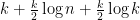 bits in the encoding. The number of strings that can be encoded using at most
  bits is
  . If we assume
  , meaning
 and
and  . We use Markov’s inequality to obtain
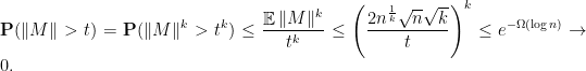
 , we need to count the number of pairs more sharply and remove the
  term, namely improve the way we talk about repetitions. Here we give an outline for how to find a tighter bound.
 is
is  vertices, that is, they have to form a tree. Furthermore, each edges is repeated exactly twice in the closed walk, otherwise we would not have enough distinct edges to connect
  distinct vertices.
 . By taking the
  . We define
 with probability
  with probability
  . Therefore
  . In fact,
  for all
  .
. .
.
 . This would give us
 . However, the bound on the number of sequences with
  , then
  w.h.p.
  .
.  , then, for every
  ,
,  . This implies that
  .
. 
 a node of degree
  .
.  and
and  for other vertices
  . We have


 ,
, 
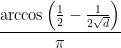
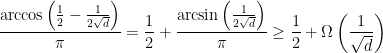
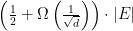
![\displaystyle cut > \frac{|E|}{2} + \Omega(n\cdot\sqrt[]{d})](https://s0.wp.com/latex.php?latex=%5Cdisplaystyle+cut+%3E+%5Cfrac%7B%7CE%7C%7D%7B2%7D+%2B+%5COmega%28n%5Ccdot%5Csqrt%5B%5D%7Bd%7D%29&bg=ffffff&fg=000000&s=0&c=20201002)
 . More generally, we will prove that you can always find a cut at least this large in the case that G is triangle-free and with maximum vertex degree
 ![\displaystyle max\ cut < \frac{|E|}{2} + O(n\cdot \sqrt[]{d})](https://s0.wp.com/latex.php?latex=%5Cdisplaystyle+max%5C+cut+%3C+%5Cfrac%7B%7CE%7C%7D%7B2%7D+%2B+O%28n%5Ccdot+%5Csqrt%5B%5D%7Bd%7D%29&bg=ffffff&fg=000000&s=0&c=20201002)

 is positive semidefinite (abbreviated PSD and written
  ) if it is symmetric and all its eigenvalues are non-negative.
  is a symmetric matrix, then all the eigenvalues of
 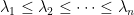 the eigenvalues of
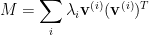
 are orthonormal eigenvectors of the
  .
. 
 .
.  , then
  if and only if the numerator
  on the right is always non-negative.
  , then
 ,
,  . By Lemma 2, this implies
  .
.  and
and  , then
 ,
,  . By Lemma 2, this implies
  , with
  , and we want to maximize, or minimize, a linear function of the variables such that linear constraints over the variables are satisfied (so far this is the same as a linear program) and subject to the additional constraint that the matrix
  is PSD. Thus, a typical semidefinite program (SDP) looks like
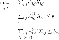
 and the scalars
  are given, and the entries of
  such that, for every
  , we have
 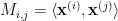 .
. 

 by setting


 are two matrices such that
  and
and  , and if
  is a scalar, then
  and
and  , and that the above optimization problem is a convex problem.
  that is satisfied by the entries of all PSD matrices but that is not satisfied by
 , then the matrix is not PSD, and the inequality
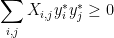
 . Thus we have a separation oracle and we can solve SDPs in polynomial time up to arbitrarily good accuracy.
 has the following equivalent characterization, as a quadratic optimization problem over real variables
  , where
  :
:
 , so that the cut edges are those with one vertex of value
  and one of value
  .
. 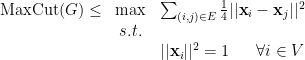

 and
and  .
.  for each vertex
  is to take a random hyperplane through the origin, and then define
  according to a rotation-invariant distribution, for example a Gaussian distribution, and let
  .
. be an edge: One sees that if
  is the angle between
  , then the probability
 ![\displaystyle \mathop{\mathbb P} [ (i,j) \mbox{ is cut } ] = \frac {\theta}{\pi}](https://s0.wp.com/latex.php?latex=%5Cdisplaystyle++%5Cmathop%7B%5Cmathbb+P%7D+%5B+%28i%2Cj%29+%5Cmbox%7B+is+cut+%7D+%5D+%3D+%5Cfrac+%7B%5Ctheta%7D%7B%5Cpi%7D+&bg=ffffff&fg=000000&s=0&c=20201002)
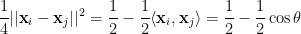
 we have
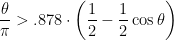
![\displaystyle \mathop{\mathbb E} [ \mbox{ number of edges cut by } (S,V-S) ] \geq .878 \cdot \sum_{(i,j) \in E} \frac 14 || {\bf x}_i - {\bf x}_j ||^2](https://s0.wp.com/latex.php?latex=%5Cdisplaystyle++%5Cmathop%7B%5Cmathbb+E%7D+%5B+%5Cmbox%7B+number+of+edges+cut+by+%7D+%28S%2CV-S%29+%5D+%5Cgeq+.878+%5Ccdot+%5Csum_%7B%28i%2Cj%29+%5Cin+E%7D+%5Cfrac+14+%7C%7C+%7B%5Cbf+x%7D_i+-+%7B%5Cbf+x%7D_j+%7C%7C%5E2+&bg=ffffff&fg=000000&s=0&c=20201002)

 .
. is a triangle-free graph in which every vertex has degree at most
 such that
  ,
, 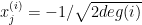 if
if  , and
, and  otherwise. We immediately see that
  for every


![{-\frac{1}{\sqrt[]{2deg(1)}}}](https://s0.wp.com/latex.php?latex=%7B-%5Cfrac%7B1%7D%7B%5Csqrt%5B%5D%7B2deg%281%29%7D%7D%7D&bg=ffffff&fg=000000&s=0&c=20201002)


![{-\frac{1}{\sqrt[]{2deg(3)}}}](https://s0.wp.com/latex.php?latex=%7B-%5Cfrac%7B1%7D%7B%5Csqrt%5B%5D%7B2deg%283%29%7D%7D%7D&bg=ffffff&fg=000000&s=0&c=20201002)


 .
. 