CS294 Lecture 1: Introduction

Posted on January 31, 2016 by luca

In which we describe what this course is about.

1. Overview

This is class is about applications of linear algebra to graph theory and to graph algorithms. In the finite-dimensional case, linear algebra deals with vectors and matrices, and with a number of useful concepts and algorithms, such as determinants, eigenvalues, eigenvectors, and solutions to systems of linear equations.

The application to graph theory and graph algorithms comes from associating, in a natural way, a matrix to a graph ${G=(V,E)}$ , and then interpreting the above concepts and algorithms in graph-theoretic language. The most natural representation of a graph as a matrix is via the ${|V| \times |V|}$ adjacency matrix of a graph, and certain related matrices, such as the Laplacian and normalized Laplacian matrix will be our main focus. We can think of ${|V|}$ -dimensional Boolean vectors as a representing a partition of the vertices, that is, a cut in the graph, and we can think of arbitrary vectors as fractional cuts. From this point of view, eigenvalues are the optima of continuous relaxations of certain cut problems, the corresponding eigenvectors are optimal solutions, and connections between spectrum and cut structures are given by rounding algorithms converting fractional solutions into integral ones. Flow problems are dual to cut problems, so one would expect linear algebraic techniques to be helpful to find flows in networks: this is the case, via the theory of electrical flows, which can be found as solutions to linear systems.

The course can be roughly subdivided into three parts: in the first part of the course we will study spectral graph algorithms, that is, graph algorithms that make use of eigenvalues and eigenvectors of the normalized Laplacian of the given graph. In the second part of the course we will look at constructions of expander graphs, and their applications. In the third part of the course, we will look at fast algorithms for solving systems of linear equations of the form ${L {\bf x} = {\bf b}}$ , where ${L}$ is Laplacian of a graph, their applications to finding electrical flows, and the applications of electrical flows to solving the max flow problem.

Continue reading →

Course on spectral methods and expanders

Posted on January 19, 2016 by luca

This semester, starting tomorrow, I am teaching a course on spectral methods and expanders. This is similar to a course I offered twice at Stanford, but this time it will be a 15-week course instead of a 10-week one.

The Stanford course had two main components: (1) spectral algorithms for sparsest cut, and comparisons with LP and SDP based methods, and (2) properties and constructions of expanders.

I will use the additional time to talk a bit more about spectral algorithms, including clustering algorithms, and about constructions of expanders, and to add a third part about electrical networks, sparsification, and max flow.

Lecture notes will be posted here after each lecture.

In some more detail, the course will start with a review of linear algebra and a proof of basic spectral graph theory facts, such as the multiplicity of 0 as an eigenvalue of the Laplacian being the same as the number of connected components of a graph.

Then we will introduce expansion and conductance, and prove Cheeger’s inequality. We will do so in the language of approximation algorithms, and we will see how the analysis of Fiedler’s algorithm given by Cheeger’s inequality compares to the Leighton-Rao analysis of the LP relaxation and the Arora-Rao-Vazirani analysis of the SDP relaxation. Then we will prove several variants of Cheeger’s inequality, interpreting them as analyses of spectral algorithms for clustering and max cut.

In the second part of the course, we will see properties of expanders and combinatorial and algebraic constructions of expanders. We will talk about the theory that gives eigenvalues and eigenvectors of Abelian Cayley graphs, the zig-zag graph product, and the Margulis-Gabber-Galil construction. I would also like to talk about the expansion of random graphs, and to explain how one gets expander constructions from Selberg’s “3/16 theorem,” although I am not sure if there will be time for that.

The first two parts will be tied together by looking at the MCMC algorithm to approximate the number of perfect matchings in a dense bipartite graph. The analysis of the algorithm depends on the mixing time of a certain exponentially big graph, the mixing time will be determined (as shown in a previous lecture on properties of expanders) by the eigenvalue gap, the eigenvalue gap will be determined (as shown by Cheeger’s inequality) by the conductance, and the conductance can be bounded by constructing certain multicommodity flows (as shown in the analysis of the Leighton-Rao algorithms).

In the third part, we will talk about electrical networks, effective resistance and electrical flows, see how to get sparsifiers using effective resistance, a sketch of how to salve Laplacian equations in nearly linear time, and how to approximate max flow using electrical flows.

Harald Helfgott on Growth in Groups

Posted on February 20, 2015 by luca

The Bulletin of the AMS is going to publish a 57-page survey on growth in groups, which is already online, and which touches several topics of interest to readers of in theory, including the recent work of Bourgain and Gamburd on expander Cayley graphs of $SL_2(p)$ and the work of Helfgott and Seress on the diameter of permutation groups.

Riemann zeta functions and linear operators

Posted on September 22, 2014 by luca

A conjectural approaches to the Riemann hypothesis is to find a correspondence between the zeroes of the zeta function and the eigenvalues of a linear operator. This was first conceived by Hilbert and by Pólya in the 1910s. (See this correspondence with Odlyzko.) In the subsequent century, there have been a number of rigorous results relating the zeroes of zeta functions in other settings to eigenvalues of linear operators. There is also a connection between the distribution of known zeroes of the Riemann zeta function, as derived from explicit calculations, and the distribution of eigenvalues of the Gaussian unitary ensemble.

In a previous post we talked about the definition of the Ihara zeta function of a graph, and Ihara’s explicit formula for it, in terms of a determinant that is closely related to the characteristic polynomial of the adjacency matrix of the graph, so that the zeroes of the zeta function determine the eigenvalue of the graph. And if the zeta function of the graph satisfies a “Riemann hypothesis,” meaning that, after a change of variable, all zeroes and poles of the zeta function are ${1/\sqrt {d-1}}$ in absolute value, then the graph is Ramanujan. Conversely, if the graph is Ramnujan then its Ihara zeta function must satisfy the Riemann hypothesis.

As I learned from notes by Pete Clark, the zeta functions of curves and varieties in finite fields also involve a determinant, and the “Riemann hypothesis” for such curves is a theorem (proved by Weil for curves and by Deligne for varieties), which says that (after an analogous change of variable) all zeroes and poles of the zeta function must be ${\sqrt q}$ in absolute value, where ${q}$ is the size of the finite field. This means that one way to prove that a family of ${(q+1)}$ -regular graphs is Ramanujan is to construct for each graph ${G_n}$ in the family a variety ${V_n}$ over ${{\mathbb F}_q}$ such that the determinant that comes up in the zeta function of ${G_n}$ is the “same” (up to terms that don’t affect the roots, and to the fact that if ${x}$ is a root for one characteristic polynomial, then ${1/x}$ has to be a root for the other) as the determinant that comes up in the zeta function of the variety ${V_n}$ . Clark shows that one can constructs such families of varieties (in fact, curves are enough) for all the known algebraic constructions of Ramanujan graphs, and one can use families of varieties for which the corresponding determinant is well understood to give new constructions. For example, for every ${d}$ , if ${k}$ is the number of distinct prime divisors of ${d-1}$ (which would be one if ${d-1}$ is a prime power) Clark gets a family of graphs with second eigenvalue ${2^k \sqrt{d-1}}$ . (The notes call ${k}$ the number of distinct prime divisors of ${d}$ , but it must be a typo.)

So spectral techniques underlie fundamental results in number theory and algebraic geometry, which then give us expander graphs. Sounds like something that we (theoretical computer scientists) should know more about.

The purpose of these notes is to explore a bit more the statements of these results, although we will not even begin to discuss their proofs.

One more reason why I find this material very interesting is that all the several applications of polynomials in computer science (to constructing error-correcting codes, secret sharing schemes, ${k}$ -wise independent generators, expanders of polylogarithmic degree, giving the codes used in PCP constructions, self-reducibility of the permanent, proving combinatorial bounds via the polynomial method, and so on), always eventually rely on three things:

A multivariate polynomial restricted to a line can be seen as a univariate polynomial (and restricting to a ${k}$ -dimensional subspace gives a ${k}$ -variate polynomial); this means that results about multivariate polynomials can often be proved via a “randomized reduction” to the univariate case;
A univariate polynomial of degree ${d}$ has at most ${d}$ roots, which follows from unique factorization
Given ${d}$ desired roots ${a_1,\ldots,a_d}$ we can always find an univariate polynomial of degree ${d}$ which has those roots, by defining it as ${\prod_i (x-a_i)}$ .

This is enough to explain the remarkable pseudo-randomness of constructions that we get out of polynomials, and it is the set of principles that underlie much of what is below, except that we are going to restrict polynomials to the set of zeroes of another polynomial, instead of a line, and this is where things get much more complicated, and interesting.

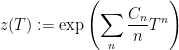
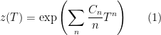
Before getting started, however, I would like to work out a toy example (which is closely related to what goes on with the Ihara zeta function) showing how an expression that looks like the one defining zeta functions can be expressed as a characteristic polynomial of a linear operator, and how its roots (which are then the eigenvalues of the operator) help give bound to a counting problem, and how one can get such bounds directly from the trace of the operator.

If we have quantities ${C_n}$ that we want to bound, then the “zeta function” of the sequence is

$\displaystyle z(T) := \exp\left( \sum_n \frac {C_n}{n} T^n \right)$

For example, and this will be discussed in more detail below, if ${P(\cdot,\cdot)}$ if a bivariate polynomial over ${{\mathbb F}_q}$ , we may be interested in the number ${C_1}$ of solutions of the equation ${P(x,y) = 0}$ over ${{\mathbb F}_q}$ , as well as the number of solutions ${C_n}$ over the extension ${{\mathbb F}_{q^n}}$ . In this case, the zeta function of the curve defined by ${P}$ is precisely

$\displaystyle z(T) = \exp\left( \sum_n \frac {C_n}{n} T^n \right) \ \ \ \ \ (1)$

and Weil proved that ${z(\cdot)}$ is a rational function, and that if ${\alpha_1,\ldots,\alpha_{2g}}$ are the zeroes and poles of ${z()}$ , that is, the roots of the numerator and the denominator, then they are all at most ${\sqrt q}$ in absolute value, and one has

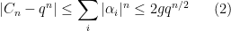
$\displaystyle | C_n - q^n | \leq \sum_i |\alpha_i|^n \leq 2g q^{n/2} \ \ \ \ \ (2)$

How does one get an approximate formula for ${C_n}$ as in (2) from the zeroes of a function like (1), and what do determinants and traces have got to do with it?

Here is our toy example: suppose that we have a graph ${G=(V,E)}$ and that ${c_\ell}$ is the number of cycles of the graph of length ${\ell}$ . Here by “cycle of length ${\ell}$ ” we mean a sequence ${v_0,\ldots,v_\ell}$ of vertices such that ${v_0=v_\ell}$ and, for ${i=0,\ldots,\ell-1}$ , ${\{ v_i,v_{i-1} \} \in E}$ . So, for example, in a graph in which the vertices ${a,b,c}$ form a triangle, ${a,b,c,a}$ and ${a,c,b,a}$ are two distinct cycles of length 3, and ${a,b,a}$ is a cycle of length 2.

We could define the function

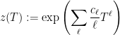
$\displaystyle z(T) := \exp\left( \sum_\ell \frac {c_\ell}{\ell} T^\ell \right)$

and hope that its zeroes have to do with the computation of ${c_\ell}$ , and that ${z}$ can be defined in terms of the characteristic polynomial.

Indeed, we have (remember, ${T}$ is a complex number, not a matrix):

$\displaystyle z(T) = \frac 1 {\det (I - TA) }$

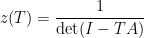
and, if ${\alpha_1,\ldots,\alpha_n}$ are the zeroes and poles of ${z(T)}$ , then

$\displaystyle c_\ell \leq \sum_i |\alpha_i|^{-\ell}$

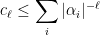
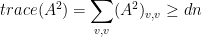
How did we get these bounds? Well, we cheated because we already knew that ${c_\ell = {\rm Tr}(A^\ell) = \sum_i \lambda_i^\ell}$ , where ${\lambda_i}$ are the eigenvalues of ${A}$ . This means that

$\displaystyle z(T) = \exp \left( \sum_\ell \sum_i \frac {\lambda_i^\ell}{\ell} T^\ell \right)$

$\displaystyle = \prod_i \exp \left( \sum_\ell \frac {\lambda_i^\ell}{\ell} T^\ell \right)$

$\displaystyle = \prod_i \frac 1 {1- T\lambda_i }$

$\displaystyle = \frac 1 { \det(I - TA) }$

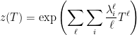
Where we used ${\frac 1 {1-x} = \exp\left( \sum_n \frac { x^n}{n} \right)}$ . Now we see that the poles of ${z}$ are precisely the inverses of the eigenvalues of ${A}$ .

Now we are ready to look more closely at various zeta functions.

I would like to thank Ken Ribet and Jared Weinstein for the time they spent answering questions. Part of this post will follow, almost word for word, this post of Terry Tao. All the errors and misconceptions below, however, are my own original creation.

Continue reading →

References on Laplacian eigenvalues and graph properties

Posted on September 20, 2014 by luca

After my lectures in the “boot camp” of the spectral graph theory program at the Simons Institute, I promised I would post some references, because I stated all results without attribution.

Here is a a first draft.

If you notice that work that you know of (for example, your work) is misrepresented or absent, please let me know and I will edit the document. (If possible, when you do so, do not compare me to Stalin and cc your message to half a dozen prominent people — true story.)

The expansion of the Paley graph

Posted on September 10, 2014 by luca

Suppose that we want to construct a very good family of ${d}$ -regular expander graphs. The Alon-Boppana theorem says that the best we can hope for, from the point of view of spectral expansion, is to have ${\lambda_2 \leq 2 \sqrt{d-1}}$ , and we would certainly be very happy with a family of graphs in which ${\lambda_2 \leq O(\sqrt d)}$ .

Known constructions of expanders produce Cayley graphs (or sometimes Schreier graphs, which is a related notion), because it is easier to analyze the spectra of such graphs. If ${\Gamma}$ is a group with operation ${\cdot}$ and ${a^{-1}}$ is the inverse of element ${a}$ , and ${S}$ is a symmetric set of generators, then the Cayley graph ${Cay(\Gamma, S)}$ is the graph whose vertices are the elements of ${\Gamma}$ and whose edges are the pairs ${(a,b)}$ such that ${a\cdot b^{-1} \in S}$ .

When the group is Abelian, there is good news and bad news. The good news is that the eigenvectors of the graphs are completely characterized (they are the characters of ${\Gamma}$ ) and the eigenvalues are given by a nice formula. (See here and here.) The bad news is that constant-degree Cayley graphs of Abelian groups cannot be expanders.

That’s very bad news, but it is still possible to get highly expanding graphs of polylogarithmic degree as Cayley graphs of Abelian groups.

Here we will look at the extreme case of a family of graphs of degree ${d_n = n/2}$ , where ${n}$ is the number of vertices. Even with such high degree, the weak version of the Alon-Boppana theorem still implies that we must have ${\sigma_2 \geq \Omega(\sqrt d_n)}$ , and so we will be happy if we get a graph in which ${\sigma_2 \leq O(\sqrt d) = O(\sqrt n)}$ . Highly expanding graphs of degree ${n/2}$ are interesting because they have some of the properties of random graphs from the ${G_{n,\frac 12}}$ distribution. In turn, graphs from ${G_{n,\frac 12}}$ have all kind of interesting properties with high probabilities, including being essentially the best known Ramsey graphs and having the kind of discrepancy property that gives seedless extractors for two independent sources. Unfortunately, these properties cannot be certified by spectral methods. The graph that we will study today is believed to have such stronger properties, but there is no known promising approach to prove such conjectures, so we will content ourselves with proving strong spectral expansion.

The graph is the Paley graph. If ${p}$ is a prime, ${{\mathbb Z} / p {\mathbb Z}}$ is the group of addition modulo ${p}$ , and ${Q}$ is the set of elements of ${{\mathbb Z}/ p{\mathbb Z}}$ of the form ${r^2 \bmod p}$ , then the graph is just ${Cay ( {\mathbb Z}/p{\mathbb Z}, Q)}$ . That is, the graph has a vertex ${v}$ for each ${v\in \{ 0,\ldots,p-1\}}$ , and two vertices ${a,b}$ are adjacent if and only if there is an ${r\in \{ 0,\ldots,p-1\}}$ such that ${a-b \equiv r^2 \pmod p}$ .

Continue reading →

The Alon-Boppana Theorem

Posted on September 1, 2014 by luca

Let ${G=(V,E)}$ be a ${d}$ -regular graph, and let

$\displaystyle d= \lambda_1 \geq \lambda_2 \geq \cdots \geq \lambda_n$

be the eigenvalues of the adjacency matrix of ${A}$ counted with multiplicities and sorted in descending order.

How good can the spectral expansion of ${G}$ be?

1. Simple Bounds

The simplest bound comes from a trace method. We have

$\displaystyle trace(A^2) = \sum_i \lambda_i^2$

by using one definition of the trace and

$\displaystyle trace(A^2) = \sum_{v,v} (A^2)_{v,v} \geq dn$

using the other definition and observing that ${(A^2)_{v,v}}$ counts the paths that go from ${v}$ to ${v}$ in two steps, of which there are at least ${d}$ : follow an edge to a neighbor of ${v}$ , then follow the same edge back. (There could be more if ${G}$ has multiple edges or self-loops.)

So we have

$\displaystyle dn \leq d^2 + \sum_{i=2,\ldots,n} \lambda_i ^2$

and so

$\displaystyle \max_{i=2,\ldots,n} |\lambda_i | \geq \sqrt d \cdot \sqrt{\frac {n-d}{n-1}}$

The condition ${d \leq n(1-\epsilon)}$ is necessary to get lower bounds of ${\Omega(\sqrt d)}$ ; in the clique, for example, we have ${d=n-1}$ and ${\lambda_2 = \lambda_n = -1}$ .

A trace argument does not give us a lower bound on ${\lambda_2}$ , and in fact it is possible to have ${\lambda_2=0}$ and ${d= n/2}$ , for example in the bipartite complete graph.

If the diameter of ${G}$ is at least 4, it is easy to see that ${\lambda_2 \geq \sqrt d}$ . Let ${a,b}$ be two vertices at distance 4. Define a vector ${x}$ as follows: ${x_a = 1}$ , ${x_v = 1/\sqrt d}$ if ${v}$ is a neighbor of ${a}$ , ${x_b=-1}$ and ${x_v = - 1/\sqrt d}$ if ${v}$ is a neighbor of ${b}$ . Note that there cannot be any edge between a neighbor of ${a}$ and a neighbor of ${b}$ . Then we see that ${||x||^2 = 4}$ , that ${x^T A x \geq 4\sqrt d}$ (because there are ${2d}$ edges, each counted twice, that give a contribution of ${1/\sqrt d}$ to ${\sum_{u,v} A_{uv} x_u x_v}$ ) and that ${x}$ is orthogonal to ${(1,\ldots,1)}$ .

2. Nilli’s Proof of the Alon-Boppana Theorem

Nilli’s proof of the Alon-Boppana theorem gives

$\displaystyle \lambda_2 \geq 2 \sqrt{ d-1 } - O \left( \frac {\sqrt{d-1}}{diam(G)-4} \right)$

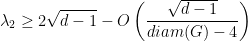
where ${diam(G) \geq \frac {\log |V|}{\log d-1}}$ is the diameter of ${G}$ . This means that if one has a family of (constant) degree- ${d}$ graphs, and every graph in the family satisfies ${\lambda_2 \leq \lambda}$ , then one must have ${\lambda \geq 2 \sqrt{d -1}}$ . This is why families of Ramanujan graphs, in which ${\lambda_2 \leq 2 \sqrt{d-1}}$ , are special, and so hard to construct, or even to prove existence of.

Friedman proves a stronger bound, in which the error term goes down with the square of the diameter. Friedman’s proof is the one presented in the Hoory-Linial-Wigderson survey. I like Nilli’s proof, even if it is a bit messier than Friedman’s, because it starts off with something that clearly is going to work, but the first two or three ways you try to establish the bound don’t work (believe me, I tried, because I didn’t see why some steps in the proof had to be that way), but eventually you find the right way to break up the estimate and it works.

So here is Nilli’s proof. Continue reading →

The Expander Mixing Lemma in Irregular Graphs

Posted on August 26, 2014 by luca

Today, after a lecture in the spectral graph theory boot camp at the Simons institute, I was asked what the expander mixing lemma is like in graphs that are not regular.

I don’t know if I will have time to return to this tomorrow, so here is a quick answer.

First, for context, the expander mixing lemma in regular graph. Say that ${G=(V,E)}$ is a ${d}$ -regular undirected graph, and ${A}$ is its adjacency matrix. Then let the eigenvalues of the normalized matrix ${\frac 1d A}$ be

$\displaystyle 1 = \lambda_1 \geq \lambda_2 \geq \cdots \geq \lambda_n$

We are interested in graphs for which all the eigenvalues are small in absolute value, except ${\lambda_1}$ , that is, if we define

$\displaystyle \sigma_2 := \max\{ |\lambda_2|, |\lambda_3 | , \ldots , | \lambda_n | \}$

we are interested in graphs for which ${\sigma_2}$ is small. The expander mixing lemma is the fact that for every two disjoint sets ${S}$ and ${T}$ of vertices we have

$\displaystyle \left | E(S,V-S) - \frac d n \cdot |S| \cdot |T| \right | \leq \sigma_2 d \sqrt{ |S| \cdot |T|} \ \ \ \ \ (1)$

The inequality (1) says that, if ${\sigma_2}$ is small, then the number of edges between every two large sets of vertices is almost determined just by the size of the sets, and it is equal to the expected number of edges between the two sets in a random ${d}$ -regular graph, up to an error term that depends on ${\sigma_2}$ .

For the proof, we observe that, if we call ${J}$ the matrix that has ones everywhere, then

$\displaystyle \sigma_2 = \max_{x \perp (1,\ldots , 1) } \frac { |x^T A x|}{d\cdot x^Tx} = \max_{x} \frac { \left|x^T \left( A - \frac dn J \right) x \right|}{d\cdot x^T x} = \max_{x,y} \frac { \left|x^T \left( A - \frac dn J \right) y \right|}{d\cdot ||x|| \cdot ||y||}$

and then we substitute ${x := {\mathbf 1}_S}$ and ${y:= {\mathbf 1}_T}$ in the above expression and do the calculations.

In the case of an irregular undirected graph ${G=(V,E)}$ , we are going to consider the normalized adjacency matrix ${M:= D^{-\frac 12} A D^{-\frac 12 }}$ , where ${A}$ is the adjacency matrix of ${G}$ and ${D}$ is the diagonal matrix such that ${D_{v,v} = d_v}$ , where ${d_v}$ is the degree of ${v}$ . As in the regular case, the eigenvalues of the normalized adjacency matrix satisfy

$\displaystyle 1 = \lambda_1 \geq \lambda_2 \geq \cdots \lambda_n \geq -1$

Let us define

$\displaystyle \sigma_2:= \max \{ |\lambda_2| , |\lambda_3| , \ldots, |\lambda_n| \}$

the second largest eigenvalue in absolute value of ${M}$ .

We will need two more definitions: for a set of vertices ${S}$ , its volume is defined as

$\displaystyle vol(S):= \sum_{v\in S} d_v$

the sum of the degrees and ${\bar d = \frac 1n \sum_v d_v}$ the average degree, so that ${vol(V) = \bar d n }$ . Now we have

Lemma 1 (Expander Mixing Lemma) For every two disjoint sets of vertices ${S}$ , ${T}$ , we have

$\displaystyle \left | E(S,V-S) - \frac {vol(S) \cdot vol(T) }{vol(V)} \right | \leq \sigma_2 \sqrt{vol(S) \cdot vol(T) } \ \ \ \ \ (2)$

So, once again, we have that the number of edges between ${S}$ and ${T}$ is what one would expect in a random graph in which the edge ${(u,v)}$ exists with probability ${d_ud_v/vol(V)}$ , up to an error that depends on ${\sigma_2}$ .

Continue reading →

The spectrum of the infinite tree

Posted on August 20, 2014 by luca

The spectral norm of the infinite ${d}$ -regular tree is ${2 \sqrt {d-1}}$ . We will see what this means and how to prove it.

When talking about the expansion of random graphs, abobut the construction of Ramanujan expanders, as well as about sparsifiers, community detection, and several other problems, the number ${2 \sqrt{d-1}}$ comes up often, where ${d}$ is the degree of the graph, for reasons that tend to be related to properties of the infinite ${d}$ -regular tree.

Continue reading →

The Riemann hypothesis for graphs

Posted on August 18, 2014 by luca

A regular connected graph is Ramanujan if and only if its Ihara zeta function satisfies a Riemann hypothesis.

The purpose of this post is to explain all the words in the previous sentence, and to show the proof, except for the major step of proving a certain identity.

There are at least a couple of reasons why more computer scientists should know about this result. One is that it is nice to see a connection, even if just at a syntactic level, between analytic facts that imply that the primes are pseudorandom and analytic facts that imply that good expanders are pseudorandom (the connection is deeper in the case of the Ramanujan Cayley graphs constructed by Lubotzky, Phillips and Sarnak). The other is that the argument looks at eigenvalues of the adjacency matrix of a graph as roots of a characteristic polynomial, a view that is usually not very helpful in achieving quantitative result, with the important exception of the work of Marcus, Spielman and Srivastava on interlacing polynomials.

Continue reading →

in theory

"Marge, I agree with you – in theory. In theory, communism works. In theory." — Homer Simpson

Tag Archives: Expanders

CS294 Lecture 1: Introduction

Course on spectral methods and expanders

Harald Helfgott on Growth in Groups

Riemann zeta functions and linear operators

References on Laplacian eigenvalues and graph properties

The expansion of the Paley graph

The Alon-Boppana Theorem

The Expander Mixing Lemma in Irregular Graphs

The spectrum of the infinite tree

The Riemann hypothesis for graphs