Online convex optimization deals with the following setup: we want to design an algorithm that, at each discrete time step  , comes up with a solution
  , where
  is a certain convex set of feasible solution. After the algorithm has selected its solution
  , a convex cost function
  , coming from a known restricted set of admissible cost functions
  , is revealed, and the algorithm pays the loss
  .
.
Again, the algorithm has to come up with a solution without knowing what cost functions it is supposed to be optimizing. Furthermore, we will think of the sequence of cost functions  not as being fixed in advanced and unknown to the algorithm, but as being dynamically generated by an adversary, after seeing the solutions provided by the algorithm. (This resilience to adaptive adversaries will be important in most of the applications.)
The offline optimum after  steps is the total cost that the best possible fixed solution would have incurred when evaluated against the cost functions seen by the algorithm, that is, it is a solution to

The regret after steps is the difference between the loss suffered by the algorithm and the offline optimum, that is,
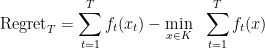
The remarkable results that we will review give algorithms that achieve regret
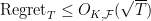
that is, for fixed and , the regret-per-time-step goes to zero with the number of steps, as  . It is intuitive that our bounds will have to depend on how big is the “diameter” of and how large is the “magnitude” and “smoothness” of the functions
  , but depending on how we choose to formalize these quantities we will be led to define different algorithms.


In the adversary setting, and with a fixed x, isn’t the offline optimum simply $T\min_{x\in K}\max_{f\in\mathcal{F}} f(x)$?
Shouldn’t the definition of online optimum allow for different values of $x$ at different time steps? In your current form the regret can be negative, e.g. for two time steps $f_0(x)=x, f_1(x)=1-x, x_0=0, x_1=1$ the regret is $(0 + 0) – 1 = -1$.
Looking forward to this series of posts, and in particular to the applications in complexity!
A quick comment: in the OCO context, where the solution points (x_t) are chosen deterministically, the distinction between oblivious and adaptive adversaries is immaterial (they have the same power). The difference becomes meaningful only where x_t is potentially chosen at random. For OCO having a random x_t only comes into play in the limited feedback scenarios (e.g., bandit).
@Sebastian: yes, good point.
@anonymous: if you define the offline optimum as being allowed to be adaptive, then you get a notion for which it is impossible to prove interesting bounds. The notion of approximation stated here, in which the algorithm is compared to an alternative that is more powerful (because it has full knowledge of the cost functions) but also more limited (because it cannot change the solution at each step) has the right mix of being possible and being useful. And, indeed, the regret can be negative
@sapers: now you are thinking of an “offline” setup in which it is the adversary that is allowed to pick fresh cost functions, and trying to make the offline optimum as small as possible, in which case it would become a two-player zero-sum game whose optimal strategies are those you state. Maybe “offline optimum” is a poor choice of terminology, but the setup is as described: we compare the algorithm to an alternative in which the cost functions are the same, and we must pick a fixed answer to use at each step (whichever minimizes the loss).