Online Optimization Post 1: Multiplicative Weights

The multiplicative weights or hedge algorithm is the most well known and most frequently rediscovered algorithm in online optimization.

The problem it solves is usually described in the following language: we want to design an algorithm that makes the best possible use of the advice coming from ${n}$ self-described experts. At each time step ${t=1,2,\ldots}$ , the algorithm has to decide with what probability to follow the advice of each of the experts, that is, the algorithm has to come up with a probability distribution ${x_t = (x_t(1),\ldots,x_t(n))}$ where ${x_t (i) \geq 0}$ and ${\sum_{i=1}^n x_t(i)=1}$ . After the algorithm makes this choice, it is revealed that following the advice of expert ${i}$ at time ${t}$ leads to loss ${\ell_t (i)}$ , so that the expected loss of the algorithm at time ${t}$ is ${\sum_{i=1}^n x_t(i) \ell_t (i)}$ . A loss can be negative, in which case its absolute value can be interpreted as a profit.

After ${T}$ steps, the algorithm “regrets” that it did not just always follow the advice of the expert that, with hindsight, was the best one, so that the regret of the algorithm after ${T}$ steps is

$\displaystyle {\rm Regret}_T = \left( \sum_{t=1}^T\sum_{i=1}^n x_t(i) \ell_t(i) \right) - \left( \min_{i=1,\ldots,n} \ \ \sum_{t=1}^T \ell_t(i) \right)$

This corresponds to the instantiation of the framework we described in the previous post to the special case in which the set of feasible solutions ${K}$ is the set ${\Delta \subseteq {\mathbb R}^n}$ of probability distributions over the sample space ${\{ 1,\ldots,n\}}$ and in which the loss functions ${f_t (x)}$ are linear functions of the form ${f_t (x) = \sum_i x(i) \ell_t (i)}$ . In order to bound the regret, we also have to bound the “magnitude” of the loss functions, so in the following we will assume that for all ${t}$ and all ${i}$ we have ${| \ell_t (i) | \leq 1}$ , and otherwise we can scale everything by a known upper bound on ${\max_{t,i} |\ell_t |}$ .

We now describe the algorithm.

The algorithm maintains at each step ${t}$ a vector of weights ${w_t = (w_t(1),\ldots,w_t(n))}$ which is initialized as ${w_1 := (1,\ldots,1)}$ . The algorithm performs the following operations at time ${t}$ :

${w_t (i) := w_{t-1} (i) \cdot e^{-\epsilon \ell_{t-1} (i) }}$
${x_t (i) := \displaystyle \frac {w_t (i) }{\sum_{j=1}^n w_t(j) }}$

That is, the weight of expert ${i}$ at time ${t}$ is ${e^{-\epsilon \sum_{k=1}^{t-1} \ell_k (i)}}$ , and the probability ${x_t(i)}$ of following the advice of expert ${i}$ at time ${t}$ is proportional to the weight. The parameter ${\epsilon>0}$ is hardwired into the algorithm and we will optimize it later. Note that the algorithm gives higher weight to experts that produced small losses (or negative losses of large absolute value) in the past, and thus puts higher probability on such experts.

We will prove the following bound.

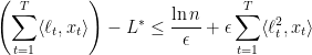
Theorem 1 Assuming that for all ${t}$ and ${i}$ we have ${| \ell_t(i) | \leq 1}$ , for every ${0 < \epsilon < 1/2}$ , after ${T}$ steps the multiplicative weight algorithm experiences a regret that is always bounded as

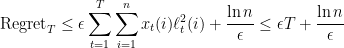
$\displaystyle {\rm Regret}_T \leq \epsilon \sum_{t=1}^T \sum_{i=1}^n x_t(i) \ell^2 _t (i) + \frac {\ln n}{\epsilon} \leq \epsilon T + \frac {\ln n}{\epsilon}$

In particular, if ${T > 4 \ln n}$ , by setting ${\epsilon = \sqrt{\frac{\ln n}{T}}}$ we achieve a regret bound

$\displaystyle {\rm Regret}_T \leq 2 \sqrt{T \ln n}$

We will start by giving a short proof of the above theorem.

For each time step ${t}$ , define the quantity

$\displaystyle W_t := \sum_{i=1}^n w_t(i) \ .$

We want to prove that, roughly speaking, the only way for an adversary to make the algorithm incur a large loss is to produce a sequence of loss functions such that even the best expert incurs a large loss. The proof will work by showing that if the algorithm incurs a large loss after ${T}$ steps, then ${W_{T+1}}$ is small, and that if ${W_{T+1}}$ is small, then even the best expert incurs a large loss.

Let us define

$\displaystyle L^* = \min_{i = 1,\ldots, n} \sum_{t=1}^T \ell_t (i)$

to be the loss of the best expert. Then we have

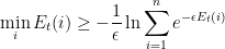
Lemma 2 (If ${W_{T+1}}$ is small, then ${L^*}$ is large)

$\displaystyle W_{T+1} \geq e^{-\epsilon L^*}$

Proof: Let ${j}$ be an index such that ${L^* = \sum_{t=1}^T \ell_t (j)}$ . Then we have

$\displaystyle W_{T+1} = \sum_{i=1}^n e^{-\epsilon \sum_{t=1}^T \ell_t(i) } \geq e^{-\epsilon \sum_{t=1}^T \ell_t(j)} = e^{-\epsilon L^*}$

$\Box$

Lemma 3 (If the loss of the algorithm is large then ${W_{T+1}}$ is small)

$\displaystyle W_{T+1} \leq n \prod_{t=1}^n (1 - \epsilon \langle x_t , \ell_t \rangle + \epsilon^2 \langle x_t , \ell^2_t \rangle)$

where ${\ell_t^2}$ is the vector whose ${i}$ -th coordinate is ${\left( \ell_t (i)\right)^2 }$

Proof: Since we know that ${W_1 = n}$ , it is enough to prove that, for every ${t=1,\ldots, T}$ , we have

$\displaystyle W_{t+1} \leq (1 - \epsilon \langle x_t , \ell_t \rangle + \epsilon^2 \langle x_t, \ell_t^2 \rangle ) \cdot W_t \ \ \ \ \ (1)$

And we see that

$\displaystyle \frac{W_{t+1}}{W_t} = \sum_{i=1}^n \frac {w_{t+1}(i)}{W_t}$

$\displaystyle = \sum_{i=1}^n \frac {w_t(i) \cdot e^{-\epsilon \ell_t (i) } }{W_t}$

$\displaystyle = \sum_{i=1}^n x_t(i) \cdot e^{-\epsilon \ell_t(i) }$

$\displaystyle \leq \sum_{i=1}^n x_t(i) \cdot ( 1 - \epsilon \ell_t (i) + \epsilon^2 \ell_t^2(i) )$

$\displaystyle = 1 - \epsilon \langle x_t, \ell_t \rangle + \epsilon^2 \langle \ell_t^2 , x_t \rangle$

where we used the definitions of our quantities and the fact that ${e^{-z} \leq 1-z+z^2}$ for ${|z| \leq 1/2}$ . $\Box$

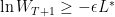
Using the fact that ${1-z \leq e^{-z}}$ for all ${|z| \leq 1}$ , the above lemmas can be restated as

$\displaystyle \ln W_{T+1} \leq \ln n - \left(\sum_{t=1}^T \epsilon \langle \ell_t , x_t \rangle \right) + \left( \sum_{t=1}^T\epsilon^2 \langle \ell_t^2 x_t\rangle \right)$

and

$\displaystyle \ln W_{T+1} \geq - \epsilon L^*$

which together imply

$\displaystyle \left( \sum_{t=1}^T \langle \ell_t , x_t \rangle \right) - L^* \leq \frac{\ln n}{\epsilon} + \epsilon \sum_{t=1}^T \langle \ell^2_t , x_t \rangle$

as desired.

Personally, I find all of the above very unsatisfactory, because both the algorithm and the analysis, but especially the analysis, seem to come out of nowhere. In fact, I never felt that I actually understood this analysis until I saw it presented as a special case of the Follow The Regularized Leader framework that we will discuss in a future post. (We will actually prove a slightly weaker bound, but with a much more satisfying proof.)

Here is, however, a story of how a statistical physicist might have invented the algorithm and might have come up with the analysis. Let’s call the loss caused by expert ${i}$ after ${t-1}$ steps the energy of expert ${i}$ at time ${t}$ :

$\displaystyle E_t(i) = \sum_{k=1}^{t-1} \ell_k(i)$

Note that we have defined it in such a way that the algorithm knows ${E_t(i)}$ at time ${t}$ . Our offline optimum is the energy of the lowest energy expert at time ${T+1}$ , that, is, the energy of the ground state at time ${T+1}$ . When we have a collection of numbers ${E_t(1),\ldots, E_t(n)}$ , a nice lower bound to their minimum is

$\displaystyle \min_i E_t(i) \geq - \frac 1 \epsilon \ln \sum_{i=1}^n e^{-\epsilon E_t(i) }$

which is true for every ${\epsilon >0}$ . The right-hand side above is the free energy at temperature ${\frac 1 \epsilon}$ at time ${t}$ . This seems like the kind of expression that we could use to bound the offline optimum, so let’s give it a name

$\displaystyle \Phi_t := - \frac 1 \epsilon \ln \sum_{i=1}^n e^{-\epsilon E_t(i) }$

In terms of coming up with an algorithm, all that we have got to work with at time ${t}$ are the losses of the experts at times ${1,\ldots,t-1}$ . If the adversary chooses to make one of the experts consistently much better than the others, it is clear that, in order to get any reasonable regret bound, the algorithm will have to put much of the probability mass in most of the steps on that expert. This suggests that the ${x_t}$ should put higher probability on experts that have done well in the first ${t-1}$ steps, that is ${x_t}$ should put higher probability on “lower-energy” experts. When we have a system in which, at time ${t}$ , state ${i}$ has energy ${E_t(i)}$ , a standard distribution that puts higher probability on lower energy states is the Gibbs distribution at temperature ${1/\epsilon}$ , defined as

$\displaystyle x_t(i) = \frac { e^{-\epsilon E_t (i)} }{\sum_j e^{-\epsilon E_t(j) } }$

where the denominator above is also called the partition function at time ${t}$

$\displaystyle Z_t := \sum_{j=1}^n e^{-\epsilon E_t(j) }$

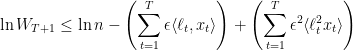
So far we have “rediscovered” our multiplicative weights algorithm, and the quantity ${W_t}$ that we had in our analysis gets interpreted as the partition function ${Z_t}$ . The fact that ${\Phi_{T+1}}$ bounds the offline optimum suggests that we should use ${\Phi_t}$ as a potential function, and aim for an analysis involving a telescoping sum. Indeed some manipulations (the same as in the short proof above, but which are now more mechanical) give that the loss of the algorithm at time ${t}$ is

$\displaystyle \langle x_t, \ell_t \rangle \leq \Phi_{t+1} - \Phi_{t} + \langle x_t , \ell^2 _t \rangle$

which telescopes to give

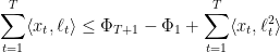
$\displaystyle \sum_{t=1}^T \langle x_t, \ell_t \rangle \leq \Phi_{T+1} - \Phi_1 + \sum_{t=1}^T\langle x_t , \ell^2 _t \rangle$

Recalling that

$\displaystyle \Phi_1 = - \frac 1 {\epsilon} \ln n$

and

$\displaystyle \Phi_{T+1} \leq \min_{j=1,\ldots, n} \sum_{t=1}^T \ell_t(j)$

we have again

$\displaystyle \left( \sum_{t=1}^T \langle x_t, \ell_t \rangle \right) - \left( \min_{j=1,\ldots, n} \sum_{t=1}^T \ell_t(j) \right) \leq \frac{\ln n}{\epsilon} + \sum_{t=1}^T\langle x_t , \ell^2 _t \rangle$

As mentioned above, we will give a better story when we get to the Follow The Regularized Leader framework. In the next post, we will discuss complexity-theory consequences of the result we just proved.

3 thoughts on “Online Optimization Post 1: Multiplicative Weights”

LK on April 24, 2019 at 11:39 pm said:

Very nice writeup!

The intuition that makes the analysis clear to me is the following:
– if an expert makes a mistake, its weight goes down by some factor.
– if we make a mistake, the _total_ weight goes down by some (other) factor.
– if we made much more mistakes than the expert, the total would go down so much that the expert’s weight would not fit in it 🙂
Ignacio Aleman on November 4, 2019 at 1:37 pm said:

Hi Luca,

I think there is a typo right after you state Lemma 3, the product goes from 1 to T (and not n) as you are iterating over time and not the experts.
Pingback: Online Optimization Post 7: Matrix Multiplicative Weights Update | in theory

Enter your comment here...

Fill in your details below or click an icon to log in:

Email (required) (Address never made public)

Name (required)

Website

You are commenting using your WordPress.com account. ( Log Out / Change )

You are commenting using your Twitter account. ( Log Out / Change )

You are commenting using your Facebook account. ( Log Out / Change )

Cancel

Connecting to %s

in theory

"Marge, I agree with you – in theory. In theory, communism works. In theory." — Homer Simpson

Online Optimization Post 1: Multiplicative Weights

3 thoughts on “Online Optimization Post 1: Multiplicative Weights”

Leave a Reply

Share this:

Like this:

Related

3 thoughts on “Online Optimization Post 1: Multiplicative Weights”

Leave a Reply