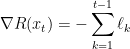
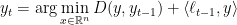
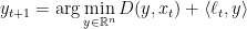
Online Optimization Post 5: Bregman Projections and Mirror Descent

In this post we return to the generic form of the FTRL online optimization algorithm. If the cost functions are linear, as they will be in all the applications that I plan to talk about, the algorithm is:

$\displaystyle x_t := \arg\min_{x\in K} \ R(x) + \sum_{k=1}^{t-1} \langle \ell_k, x \rangle \ \ \ \ \ (1)$

where $K\subseteq {\mathbb R}^n$ is the convex set of feasible solutions that the algorithm is allowed to produce, ${x \rightarrow \langle \ell_k , x \rangle}$ is the linear loss function at time ${k}$ , and ${R: K \rightarrow {\mathbb R}}$ is the strictly convex regularizer.

If we have an unconstrained problem, that is, if ${K= {\mathbb R}^n}$ , then the optimization problem (1) has a unique solution: the ${x_t}$ such that

$\displaystyle \nabla R(x_t) = - \sum_{k=1}^{t-1} \ell_k$

and we can usually both compute ${x_t}$ efficiently in an algorithm and reason about ${x_t}$ effectively in an analysis.

Unfortunately, we are almost always interested in constrained settings, and then it becomes difficult both to compute ${x_t}$ and to reason about it.

A very nice special case happens when the regularizer ${R}$ acts as a barrier function for ${K}$ , that is, the (norm of the) gradient of ${R}$ goes to infinity when one approaches the boundary of ${K}$ . In such a case, it is impossible for the minimum of (1) to occur at the boundary and the solution will be again the unique ${x_t}$ in ${K}$ such that

$\displaystyle \nabla R(x_t) = - \sum_{k=1}^{t-1} \ell_k$

We swept this point under the rug when we studied FTRL with negative-entropy regularizer in the settings of experts, in which ${K = \Delta}$ is the set of probability distributions. When we proceeded to solve (1) using Lagrange multipliers, we ignored the non-negativity constraints. The reason why it was ok to do so was that the negative-entropy is a barrier function for the non-negative orthant ${({\mathbb R}_{\geq 0})^n}$ .

Another important special case occurs when the regularizer ${R(x) = c || x||^2}$ is a multiple of length-squared. In this case, we saw that we could “decouple” the optimization problem by first solving the unconstrained optimization problem, and then projecting the solution of the unconstrained problem to ${K}$ :

$\displaystyle y_{t} = \arg\min_{y\in {\mathbb R}^n} \ c || y||^2 + \sum_{k=1}^{t-1} \langle \ell_k, y \rangle$

$\displaystyle x_t = \Pi_K (y_t) = \arg\min _{x\in K} || x - y_t ||$

Then we have the closed-form solution ${y_t = - \frac 1{2c} \sum_{k=1}^{t-1} \ell _k}$ and, depending on the set ${K}$ , the projection might also have a nice closed-form, as in the case ${K= [0,1]^n}$ that comes up in results related to regularity lemmas.

As we will see today, this approach of solving the unconstrained problem and then projecting on ${K}$ works for every regularizer, for an appropriate notion of projection called the Bregman projection (the projection will depend on the regularizer).

To define the Bregman projection, we will first define the Bregman divergence with respect to the regularizer ${R}$ , which is a non-negative “distance” ${D(x,y)}$ defined on ${{\mathbb R}^n}$ (or possibly a subset of ${{\mathbb R}^n}$ for which the regularizer ${R}$ is a barrier function). Then, the Bregman projection of ${y}$ on ${K}$ is defined as ${\arg\min_{x\in K} \ D(x,y)}$ .

Unfortunately, it is not so easy to reason about Bregman projections either, but the notion of Bregman divergence offers a way to reinterpret the FTRL algorithm from another point of view, called mirror descent. Via this reinterpretation, we will prove the regret bound

$\displaystyle {\rm Regret}_T(x) \leq D(x,x_1) + \sum_{t=1}^T D(x_t,y_{t+1})$

which carries the intuition that the regret comes from a combination of the “distance” of our initial solution from the offline optimum and of the “stability” of the algorithm, that is, the “distance” between consecutive soltuions. Nicely, the above bound measures both quantities using the same “distance” function.

1. Bregman Divergence and Bregman Projection

For a strictly convex function ${R: {\mathbb R}^n \rightarrow {\mathbb R}}$ , we define the Bregman divergence associated to ${R}$ as

$\displaystyle D_R(x,y) := R(x) - R(y) - \langle \nabla R(y), x-y \rangle$

that is, the difference between the value of ${R}$ at ${x}$ and the value of the linear approximation of ${R}$ at ${x}$ (centered at ${y}$ ). By the strict convexity of ${R}$ we have ${D_R(x,y) \geq 0}$ and ${D_R(x,y) = 0}$ iff ${x=y}$ . These properties suggest that we may think of ${D_R(x,y)}$ as a kind of “distance” between ${x}$ and ${y}$ , which is a useful intuition although it is important to keep in mind that the divergence need not be symmetric and need not satisfy the triangle inequality.

Now we show that, assuming that ${R(\cdot)}$ is well defined and strictly convex on all ${{\mathbb R}^n}$ , and that the losses are linear, the constrained optimization problem (1) can be solved by first solving the unconstrained problem and then “projecting” the solution on ${K}$ by finding the point in ${K}$ of smallest Bregman divergence from the unconstrained optimum:

$\displaystyle y_t = \arg\min _{y\in {\mathbb R}^n} \ R(y) + \sum_{k=1}^{t-1} \langle \ell_k , y \rangle$

$\displaystyle x_t = \arg\min_{x \in K} \ D_R(x,y_t)$

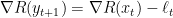
The proof is very simple. The optimum of the unconstrained optimization problem is the unique ${y_t}$ such that

$\displaystyle \nabla \left( R(y_t) + \sum_{k=1}^{t-1} \ell_k \right) = 0$

that is, the unique ${y_t}$ such that

$\displaystyle \nabla R(y_t) = - \sum_{k=1}^{t-1} \ell_k$

On the other hand, ${x_t}$ is defined as

$\displaystyle x_t = \arg\min_{x \in K} \ D_R(x,y_t) = \arg\min_{x \in K} R(x) - R(y_t) - \langle \nabla R(y_t) , x - y_t \rangle$

that is,

$\displaystyle x_t = \arg\min_{x \in K} R(x) - R(y_t) + \langle \sum_{k=1}^{t-1} \ell_k , x - y_t \rangle = \arg\min_{x \in K} R(x) + \langle \sum_{k=1}^{t-1} \ell_k , x \rangle$

where the second equality above follows from the fact that two functions that differ by a constant have the same optimal solutions.

Indeed we see that the above “decoupled” characterization of the FTRL algorithm would have worked for any definition of a function of the form

$\displaystyle D(x,y) = R(x) - \langle \nabla R(y), x \rangle + \langle \mbox{ stuff that depends only on } y \rangle$

and that our particular choice of what “stuff dependent only on ${y}$ ” to add makes ${D(x,x) = 0}$ which is reasonable for something that we want to think of as a “distance function.”

Note that, in all of the above, we can replace ${{\mathbb R}^n}$ with a convex set ${K \subseteq S \subseteq {\mathbb R}^n}$ provided that ${R}$ is a barrier function for ${S}$ . In that case

$\displaystyle y_t = \arg\min_{y\in S} R(y) + \sum_k \ell_k$

is the unique ${y_t}$ such that

$\displaystyle \nabla R(y_t) = - \sum _k \ell_k$

and everything else follows analogously.

2. Examples

2.1. Bregman Divergence of Length-Squared

If ${R(x) = ||x ||^2}$ , then

$\displaystyle D(x,y) = ||x||^2 - ||y||^2 - \langle 2 y , x- y \rangle = ||x - y||^2 \ ,$

so Bregman divergence is distance-squared, and Bregman projection is just (Euclidean) projection.

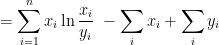
2.2. Bregman Divergence of Negative Entropy

If, for ${x\in ({\mathbb R}_{\geq 0})^n}$ , we define

$\displaystyle R(x) = \sum_{i=1}^n x_i \ln x_i$

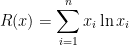
then the associated Bregman divergence is the generalized KL divergence.

$\displaystyle D(x,y) = \sum_{i=1}^n x_i \ln {x_i} \ - \sum_i y_i \ln y_i \ - \langle \nabla R(y), x-y \rangle$

where ${(\nabla R(y))_i = 1 + \ln y_i}$ so that

$\displaystyle D(x,y) = \sum_{i=1}^n x_i \ln x_i \ - \sum_i y_i \ln y_i \ - \sum_i x_i \ln y_i \ + \sum_i y_i \ln y_i \ - \sum_i x_i + \sum_i y_i$

$\displaystyle = \sum_{i=1}^n x_i \ln \frac{x_i} {y_i} \ - \sum_i x_i + \sum_i y_i$

Note that, if ${x}$ and ${y}$ are probability distributions, then the final two terms above cancel out, leaving just the KL divergence ${\sum_i x_i \ln \frac {x_i}{y_i}}$ .

3. Mirror Descent

We now introduce a new perspective on FTRL.

In the unconstrained setting, if ${R}$ is a strictly convex function and ${D}$ is the associated Bregman divergence, the mirror descent algorithm for online optimization has the update rule

$\displaystyle x_t = \arg\min_{x\in {\mathbb R}^n} D(x,x_{t-1}) + \langle \ell_{t-1}, x \rangle$

The idea is that we want to find a solution that is good for the past loss functions, but that does not “overfit” too much. If, in past steps, ${x_{t-1}}$ had been chosen to be such a solution for the loss functions ${\ell_1,\ldots,\ell_{t-2}}$ , then, in choosing ${x_t}$ , we want to balance staying close to ${x_{t-1}}$ but also doing well with respect to ${\ell_{t-1}}$ , hence the above definition.

Theorem 1 Initialized with ${x_1 = \arg\min_{x\in {\mathbb R}^n} R(x)}$ , the unconstrained mirror descent algorithm is identical to FTRL with regularizer ${R}$ .

Proof: We will proceed by induction on ${t}$ . At ${t=1}$ , the definition of ${x_1}$ is the same. For larger ${t}$ , we know that FTRL will choose the unique ${x_t}$ such that ${\nabla R(x_t) = - \sum_{k=1}^{t-1} \ell_k}$ , so we will assume that this is true for the mirror descent algorithm for ${x_{t-1}}$ and prove it for ${x_t}$ .

First, we note that the function ${x \rightarrow D(x,x_{t-1}) + \langle \ell_{t-1} , x \rangle}$ is strictly convex, because it equals

$\displaystyle R(x) - R(x_{t-1}) - \langle \nabla R(x_{t-1}), x - x_t \rangle + \langle \ell_{t-1} , x \rangle$

and so it is a sum of a strictly convex function ${R(x)}$ , linear functions in ${x}$ , and constants independent of ${x}$ . This means that ${x_t}$ is the unique point at which the gradient of the above function is zero, that is,

$\displaystyle \nabla R(x_t) - \nabla R(x_{t-1}) + \ell_{t-1} = 0$

and so

$\displaystyle \nabla R(x_t) = \nabla R(x_{t-1}) - \ell_{t-1}$

and, using the inductive hypothesis, we have

$\displaystyle \nabla R(x_t) = - \sum_{k=1}^{t-1} \ell_k$

as desired. $\Box$

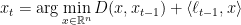
In the constrained case, there are two variants of mirror descent. Using the terminology from Elad Hazan’s survey, agile mirror descent is the natural generalization of the unconstrained algorithm:

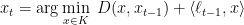
$\displaystyle x_t = \arg\min_{x\in K} \ D(x,x_{t-1}) + \langle \ell_{t-1}, x \rangle$

Following the same steps as the proof in the previous section, it is possible to show that agile mirror descent is equivalent to solving, at each iteration, the “decoupled” optimization problems

$\displaystyle y_t = \arg\min_{y\in {\mathbb R}^n} D(y,x_{t-1}) + \langle \ell_{t-1}, y \rangle$

$\displaystyle x_t = \arg\min_{x\in K} D(x,y_t)$

That is, we can first solve the unconstrained problem and then project on ${K}$ . (Again, we can always replace ${{\mathbb R}^n}$ by a set ${S}$ for which ${R}$ is a barrier function and such that ${K \subseteq S}$ .)

The lazy mirror descent algorithm has the update rule

$\displaystyle y_t = \arg\min_{x\in {\mathbb R}^n} D(y,y_{t-1}) + \langle \ell_{t-1}, y \rangle$

$\displaystyle x_t = \arg\min_{x\in K} D(x,y_t)$

The initialization is

$\displaystyle y_1 = \arg\min_{x\in {\mathbb R}^n} \ R(x) \ \ \ x_1 = \arg\min_{x\in K} R(x)$

Fact 2 Lazy mirror descent is equivalent to FTRL.

Proof: The solutions ${y_t}$ are the unconstrained optimum of FTRL, and ${x_t}$ is the Bregman projection of ${y_t}$ on ${K}$ . We proved in the previous section that this characterizes constrained FTRL. $\Box$

What about agile mirror descent? In certain special cases it is equivalent to lazy mirror descent, and hence to FTRL, but it usually leads to a different set of solutions.

We will provide an analysis of lazy mirror descent, but first we will give an analysis of the regret of unconstrained FTRL in terms of Bregman divergence, which will be the model on which we will build the proof for the constrained case.

4. A Regret Bound for FTRL in Terms of Bregman Divergence

In this section we prove the following regret bound.

Theorem 3 Unconstrained FTRL with regularizer ${R}$ satisfies the regret bound

$\displaystyle {\rm Regret}_T(x) \leq D(x,x_1) + \sum_{t=1}^T D(x_t,x_{t+1})$

where ${D}$ is the Bregman divergence associated with ${R}$ .

We will take the mirror descent view of unconstrained FTRL, so that

$\displaystyle x_1 = \arg\min_{x\in {\mathbb R}^n} \ R(x)$

$\displaystyle x_{t+1} = \arg\min_{x\in {\mathbb R}^n} \ D(x,x_t) + \langle \ell_t , x\rangle$

We proved that

$\displaystyle \nabla R(x_{t+1} ) = \nabla R(x_t) - \ell_t$

This means that we can rewrite the regret suffered at step ${t}$ with respect to ${x}$ as

$\displaystyle \langle \ell_t , x_t - x \rangle = \langle \nabla R(x_t) - \nabla R(x_{t+1}), x_t - x \rangle$

$\displaystyle = D(x,x_t) - D(x,x_{t+1} ) +D(x_t, x_{t+1})$

and the theorem follows by adding up the above expression for ${t=1,\ldots,T}$ and recalling that ${D(x,x_{T+1}) \geq 0}$ .

Unfortunately I have no geometric intuition about the above identity, although, as you can check yourself, the algebra works neatly.

5. A Regret Bound for Agile Mirror Descent

In this section we prove the following generalization of the regret bound from the previous section.

Theorem 4 Agile mirror descent satisfies the regret bound

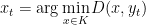
$\displaystyle {\rm Regret}_T(x) \leq D(x,x_1) + \sum_{t=1}^T D(x_t,y_{t+1})$

The first part of the update rule of agile mirror descent is

$\displaystyle y_{t+1} = \arg\min_{y\in {\mathbb R}^n} D(y,x_{t}) + \langle \ell_{t}, y \rangle$

and, following steps that we have already carried out before, ${y_{t+1}}$ satisfies

$\displaystyle \nabla R(y_{t+1} ) = \nabla R(x_t) - \ell_t$

This means that we can rewrite the regret suffered at step ${t}$ with respect to ${x}$ as

$\displaystyle \langle \ell_t , x_t - x \rangle = \langle \nabla R(x_t) - \nabla R(y_{t+1}), x_t - x \rangle$

$\displaystyle = D(x,x_t) - D(x,y_{t+1} ) +D(x_t, y_{t+1})$

where the same mystery cancellations as before make the above identity true.

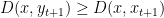
Now I will wield another piece of magic, and I will state without proof the following fact about Bregman projections

Lemma 5 If ${x\in K}$ and ${z}$ is the Bregman projection on ${K}$ of a point ${y}$ , then

$\displaystyle D(x,y) \geq D(x,z) + D(z,y)$

That is, if we think of ${D}$ as a “distance,” the distance from ${y}$ to its closest point ${z}$ in ${K}$ plus the distance from ${z}$ to ${x}$ is at most the distance from ${y}$ to ${x}$ . Note that this goes in the opposite direction as the triangle inequality (which ok, because ${D}$ typically does not satisfy the triangle inequality).

In particular, the above lemma gives us

$\displaystyle D(x,y_{t+1}) \geq D(x,x_{t+1})$

and so

$\displaystyle \langle \ell_t , x_t - x \rangle \leq D(x,x_t) - D(x,x_{t+1} ) +D(x_t, y_{t+1})$

Now summing over ${t}$ and recalling that ${D(x,x_{T+1}) \geq 0}$ we have our theorem.

2 thoughts on “Online Optimization Post 5: Bregman Projections and Mirror Descent”

Cengizhan Kuyrukcu on July 8, 2019 at 5:57 am said:

Teşekkür ederim.
http://www.webdunya.com
Pingback: Online Optimization Post 7: Matrix Multiplicative Weights Update | in theory

Enter your comment here...

Fill in your details below or click an icon to log in:

Email (required) (Address never made public)

Name (required)

Website

You are commenting using your WordPress.com account. ( Log Out / Change )

You are commenting using your Twitter account. ( Log Out / Change )

You are commenting using your Facebook account. ( Log Out / Change )

Cancel

Connecting to %s

in theory

"Marge, I agree with you – in theory. In theory, communism works. In theory." — Homer Simpson

Online Optimization Post 5: Bregman Projections and Mirror Descent

2 thoughts on “Online Optimization Post 5: Bregman Projections and Mirror Descent”

Leave a Reply

Share this:

Like this:

Related

2 thoughts on “Online Optimization Post 5: Bregman Projections and Mirror Descent”

Leave a Reply